These notes cover basic knowledge in linear algebra, statistics and probability, and machine learning, based on the CS229: Machine Learning course. While preparing for my PhD interview, I compiled these notes, deliberately omitting certain topics that seemed unlikely to be covered in the interview (which turned out to be true). Given my limited experience, there may be some errors in these notes. If you notice any mistakes or have suggestions for improvement, please feel free to email me. My contact information is available on my homepage.

References:

• Linear Algebra: Click me
• Probability Theory: Click me
• Machine Learning: Click me

A special thanks to everyone involved in creating and maintaining this course, for making it open and freely accessible.

Authored by Bingkui Tong
December 19, 2024

Linear Algebra

English	中文	Complementary
transpose	转置	$(AB{)}^T=B^T{A}^T|(A+B{)}^T=A^T+B^T$$(AB)^T=B^TA^T | (A+B)^T=A^T+B^T$
column vector	列向量	一般向量认为只有一列的矩阵
row vector	行向量	一般用列向量的转置表示行向量
product	积	比如两个矩阵相乘的结果
inner / dot product	内积/点积	两个向量相乘的结果（常数）
coefficient	系数
associative	结合律	(AB)C = A(BC)
distributive	分离律	A(B+C) = AB + AC
commutative	交换律	AB = BA (For matrix multiplication generally no)
identity matrix	单位矩阵	对角线全为1，非对角线为0
diagonal matrix	对角矩阵	除了对角线全为0
symmetric	对称的 (only for square matrix)	$A=A^T$$A=A^T$, For any matric $A\in R^{n\times n}$$A \in R^{n \times n}$, $A+A^T$$A+A^T$ is symmetric
anti-symmetric	反对称的 (only for square matrix)	$A=-A^T$$A=-A^T$, For any matric $A\in {\mathbb{R}}^{n\times n}$$A \in \mathbb{R}^{n \times n}$, $A-A^T$$A-A^T$ is anti-symmetric
		For any matric $A\in R^{n\times n}$$A \in R^{n \times n}$ can be represented as: $A=\frac{1}{2}(A+A^T)+\frac{1}{2}(A-A^T)$$A=\frac{1}{2}(A+A^T)+\frac{1}{2}(A-A^T)$, The first matrix on the right is symmetric and the second is anti-symmetric
trace	迹 (only for square matrix)	对角线元素之和$\text{tr}A=\sum _{i=1}^n{A}_{ii}$$\text{tr}A=\sum_{i=1}^{n} A_{ii}$
		对于方阵AB，$\text{tr}AB=\text{tr}BA$$\text{tr}AB=\text{tr}BA$, no matter how matrix times, it still works
square matrix	方阵
norm	范数 (only for vector)	欧几里得范数（Euclidean or ${\ell }_2$$\ell_2$norm）为$\parallel x{\parallel }_2=\sqrt{\sum _{i=1}^{i=n}{x}_i^2}=\sqrt{x^{T}x}$$\|x\|_2=\sqrt{\sum_{i=1}^{i=n}x_i^2}= \sqrt{x^Tx}$
		The four properties a norm should be satisfied: non-negativity, definiteness, homogeneity, triangle inequality
		${\ell }_p$$\ell_p$ norm is $(\sum _{i=1}^n|x_i{|}^p{)}^{\frac{1}{p}}$$(\sum_{i=1}^{n}|x_i|^p)^\frac{1}{p}$
linear independent	线性无关性	For a set of vectors {$x_1,x_2,...,x_n$$x_1, x_2, ... , x_n$}, if no vector can be represented as a linear combination of the remain vectors, we can say this vector is linear independent.
		Linear dependent: $x_n=\sum _{i=1}^{n-1}{\alpha }_i{x}_i$$x_n=\sum_{i=1}^{n-1}\alpha_ix_i$, if some scalar $\alpha$$\alpha$ make it works
rank	秩	$rank(A)$$rank(A)$: Row rank is equal to column rank, row or column rank can all be called rank
row rank	行秩	The size of largest subset of rows of A that constitute a linearly independent set The number of linearly independent rows
column rank	列秩	The size of largest subset of columns of A that constitute a linearly independent set The number of linearly independent columns
		For $A\in {\mathbb{R}}^{m\times n},rank(A)\le min(m,n)$$A\in \mathbb{R}^{m\times n},rank(A)\le min(m,n)$. If $rank(A)=min(m,n)$$rank(A) = min(m, n)$, we call this matrix full rank
		$\begin{array}{c}rank(AB)\le min(rank(A),rank(B))\\ rank(A+B)\le rank(A)+rank(B)\end{array}$$rank(AB)\le min(rank(A), rank(B))\\rank(A+B)\le rank(A)+rank(B)$
inverse	逆 (only for square matrix)	The inverse of $A$$A$ is $A^{-1}$$A^{-1}$, and $A{A}^{-1}=I=A^{-1}A$$AA^{-1}=I=A^{-1}A$ Not all matrices have inverses
invertible/non-singular	可逆/非奇异	A must be full rank to have an inverse
non-invertible/singular	不可逆/奇异	$\begin{array}{c}(AB{)}^{-1}=B^{-1}{A}^{-1}\\ (A^T{)}^{-1}=(A^{-1}{)}^T\end{array}$$(AB)^{-1}=B^{-1}A^{-1}\\(A^T)^{-1}=(A^{-1})^T$
orthogonal matrix	正交矩阵	Vectors: x and y is orthogonal if $x^{T}y=0$$x^Ty=0$ Matrix: a square matrix $U$$U$ is orthogonal if its all columns are orthogonal to each other and normalized (all the columns are referred to as being orthonormal)
normalized	归一化	$U^{T}U=I=U{U}^T$$U^TU=I=UU^T$, in other words, the inverse of an orthogonal matrix is its transpose. Usually we use orthogonal to describe the square matrix
		$\parallel Ux{\parallel }_2=\parallel x{\parallel }_2$$\|Ux\|_2=\|x\|_2$: operating a vector with orthogonal matrix will not change its ${\ell }_2$$\ell_2$ norm
span	生成子空间/张成	The span of a set of vectors is the set of all vectors that can be expressed as a linear combination of $\{x_1,x_2,...,x_n\}$$\{x_1, x_2, ... ,x_n\}$
		if $\{x_1,..,x_n\}$$\{x_1, .. , x_n\}$ is n linearly independent vectors, and $x_i{\in }^{\mathbb{R}}n$$x_i \in ^\mathbb{R}n$, the $span(\{x_1,..,x_n\})={\mathbb{R}}^n$$span(\{x_1, .. , x_n\})=\mathbb{R}^n$
projection	投影	一个向量到另外一组向量的投影就等于这一组向量的生成子空间中与这个向量欧几里得范数的最小值
range/columnspace	列空间/值空间	$\mathcal{R}(A)=span(x_1,...,x_n),\{x_1,...,x_n\}\text{ is the columns of }A$$\mathcal{R}(A)=span(x_1, ..., x_n), \{x_1,...,x_n\}\text{ is the columns of }A$
nullspace	零空间	nullspace of a matrix means a set of vectors equal to 0 when multiplied by A. $\mathcal{N}(A)=\{x\in {\mathbb{R}}^n:Ax=0\}$$\mathcal{N}(A)=\{x\in \mathbb{R}^n: Ax=0\}$
		$\begin{array}{c}A\in {\mathbb{R}}^{m\times n}\mathcal{R}(A^T)\cap \mathcal{N}(A)=\{0\}\\ \mathcal{R}(A^T)=\mathcal{N}(A{)}^{\perp }\end{array}$$A\in \mathbb{R}^{m\times n} \ \mathcal{R}(A^T)\cap\mathcal{N}(A)=\{0\}\\\mathcal{R}(A^T)=\mathcal{N}(A)^\perp$
determinant	行列式	$detA\text{ or }|A|$$det A \text{ or } |A|$ （几何意义：我的理解就是将一对正交基构成的空间的体积（面积）放缩的倍数）
		some properties: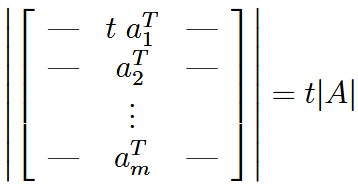 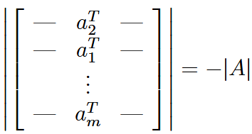$\begin{array}{c}|A|=|A^T|\\ |AB|=|A||B|\\ |A^{-1}|=\frac{1}{|A|}\end{array}$$|A|=|A^T|\\|AB|=|A||B|\\|A^{-1}|=\frac{1}{|A|}$
		full rank: determinant is not 0 / full rank (for square matrix)
		Laplace展开求行列式：$|A|=\sum _{j=1}^n(-1{)}^{i+j}{a}_{ij}|M_{ij}|\text{ ,where }{M}_{ij}\text{ is }A\text{ removed the }{i}_{th}\text{ row and }{j}_{th}\text{ column}$$|A|=\sum_{j=1}^{n}(-1)^{i+j}a_{ij}|M_{ij}|\text{ ,where }M_{ij}\text{ is }A\text{ removed the }i_{th}\text{ row and }j_{th}\text{ column}$ 这里可以任选展开一行或者一列
classical adjoint	（经典）伴随矩阵	$adj(A)\in {\mathbb{R}}^{n\times n},(adj(A){)}_{ij}=(-1{)}^{i+j}|A_{\text{}j,\text{}i}|$$adj(A)\in\mathbb{R}^{n\times n}, \ (adj(A))_{ij}=(-1)^{i+j}|A_{\textbackslash j,\textbackslash i}|$ (note that switch $i$$i$ and $j$$j$ indices in $A_{\text{}j,\text{}i}$$A_{\textbackslash j,\textbackslash i}$
		$A^{-1}=\frac{1}{|A|}adj(A)$$A^{-1}=\frac{1}{|A|}adj(A)$
quadratic form	二次形式	the scalar value $x^{T}Ax$$x^TAx$
		Usually we explicitly assume that the matrix appearing in quadratic form is symmetric 这里$A=\frac{1}{2}(A+A^T)+\frac{1}{2}(A-A^T)$$A=\frac{1}{2}(A+A^T)+\frac{1}{2}(A-A^T)$，由于最终结果是一个标量，所以这里的$A^T$$A^T$可以直接写为$A$$A$，可以看到只有左边对称的部分有贡献，右边的anti-symmetric并没有贡献
positive definite (PD)	正定	For symmetric matrix $A\in {\mathbb{S}}^n$$A\in\mathbb{S}^n$, if all non-zero vectors $x\in {\mathbb{R}}^n,x^{T}Ax>0$$x\in \mathbb{R}^n, x^TAx>0$, $A$$A$ is positive definite. Usually denoted A as $A\succ 0\text{ or just }A>0$$A \succ 0 \text{ or just } A>0$, the set of all positive definite matrices is denoted as ${\mathbb{S}}_{++}^n$$\mathbb{S}^n_{++}$
positive semidefinite (PSD)	半正定	for all vectors (not all non-zero vectors) $x$$x$, $x^{T}Ax\ge 0,A⪰0,{\mathbb{S}}_{+}^n$$x^TAx\ge0,\quad A\succeq0, \quad \mathbb{S}^n_+$
negative definite (ND)	负定	For symmetric matrix $A\in {\mathbb{S}}^n$$A\in\mathbb{S}^n$, if all non-zero vectors $x\in {\mathbb{R}}^n,x^{T}Ax<0$$x\in \mathbb{R}^n, x^TAx<0$, $A$$A$ is positive definite. Usually denoted A as $A\prec 0\text{ or just }A<0$$A \prec 0 \text{ or just } A<0$
negative semidefinite (NSD)	半负定	for all vectors (not all non-zero vectors) $x$$x$, $x^{T}Ax\le 0,A⪯0$$x^TAx\le 0,\quad A\preceq0$
indefinite	不定	neither positive semidefinite nor negative semidefinite
		positive/negative definite matrices are full rank, hence, invertible
gram matrix	格拉姆矩阵	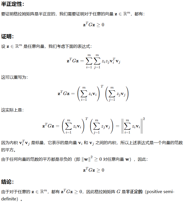$A{A}^T$$AA^T$, $A$$A$ can be in any shape and gram matrix is always positive semidefinite
eigenvalue	特征值	$Ax=\lambda x,x\ne 0$$Ax=\lambda x, x\ne 0$, where $x$$x$ is eigenvector and $\lambda$$\lambda$ is eigen value
eigenvector	特征向量	Intuitively, this definition means that multiplying $A$$A$ by the vector $x$$x$ results in a new vector that points in the same direction as $x$$x$, but scaled by a factor $\lambda$$\lambda$.
		Usually we assume the eigenvector is normalized because if $x$$x$ is eigenvector, then $ax$$ax$ is also eigenvector
		Only when $(\lambda I-A)x=0$$(\lambda I-A)x=0$ has non-empty nullspace, the x has non-zero solution (the left part columns are not linearly independent), which is only the case if $(\lambda I-A)$$(\lambda I-A)$ is singular, which means $|(\lambda I-A)|=0$$|(\lambda I-A)|=0$
		Some properties: $\begin{array}{c}trA=\sum _{i=1}^n{\lambda }_i\\ |A|=\prod _{i=1}^n{\lambda }_i\end{array}$$trA=\sum_{i=1}^n\lambda_i\\|A|=\prod_{i=1}^n\lambda_i$一个矩阵可以变成A=PDP^-1，P是可逆矩阵，D的对角线都是特征值。trA=trDPP-1=trD=sum lambda，行列式同理detA=detPDP-1=detP detD detP-1=detD 逆矩阵的特征值是原矩阵的倒数 The eigenvalues of a diagonal matrix are just the diagonal entries
diagonalizable	可对角化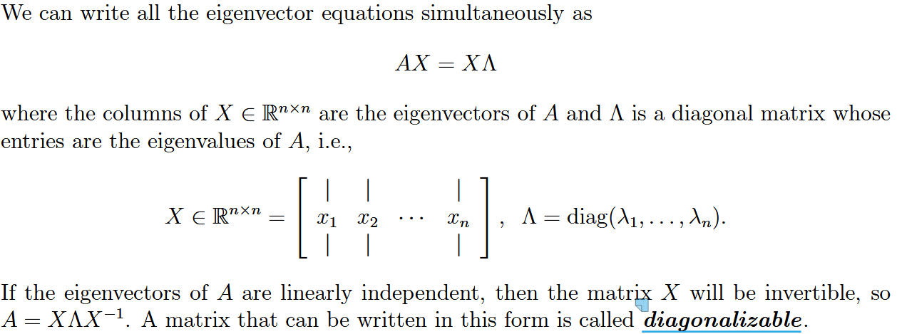
		可逆矩阵的特征值数量为n（维度），不可逆矩阵行列式为0，因为有特征值为0
Hessian	Hessian 矩阵	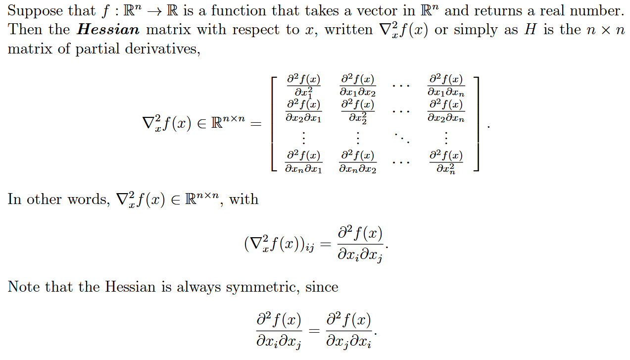就是个二阶导矩阵
least square	最小二乘法	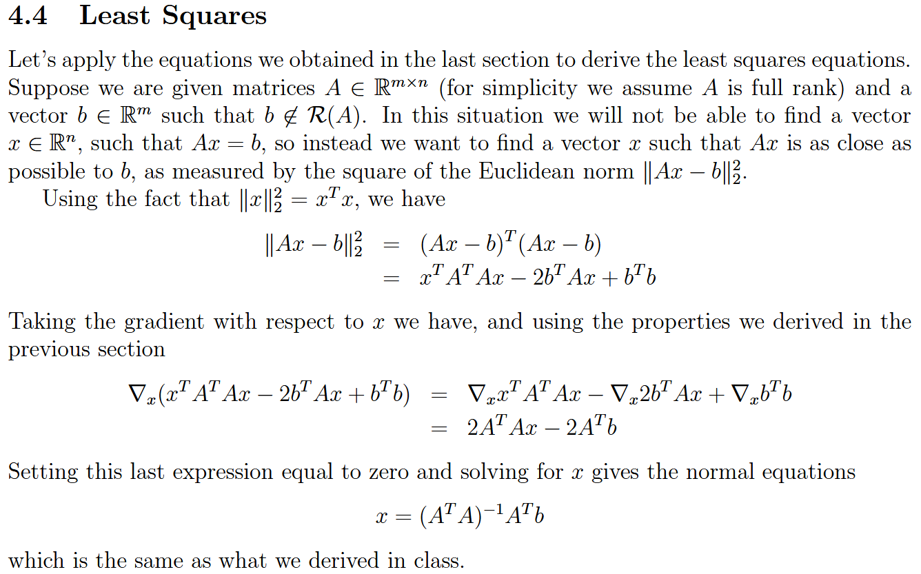使用了这两个公式

Statistics and Probability

English	中文	Complementary
sample space	样本空间	$\mathrm{\Omega }$$\Omega$: The set of all the outcomes of a random experiment
set of events (event space)	事件集（事件空间）	$\mathcal{F}$$\mathcal{F}$: properties: $\begin{array}{c}\mathrm{\varnothing }\in \mathcal{F}\\ A\in \mathcal{F}⟹\mathrm{\Omega }\text{}A\in \mathcal{F}\\ A_1,A_2,...\in \mathcal{F}⟹{\cup }_i{A}_i\in \mathcal{F}\end{array}$$\emptyset \in \mathcal{F}\\ A\in\mathcal{F}\Longrightarrow\Omega\textbackslash A\in\mathcal{{F}}\\A_1,A_2,...\in\mathcal{F}\Longrightarrow\cup_iA_i\in\mathcal{F}$
conditional probability	条件概率	$P(A|B)\triangleq \frac{P(A\cap B)}{P(B)}$$P(A|B)\triangleq\frac{P(A\cap B)}{P(B)}$
independent	独立	$P(A\cap B)=P(A)P(B)\text{ or }P(A|B)=P(A)$$P(A\cap B)=P(A)P(B) \text{ or } P(A|B)=P(A)$
random variables	随机变量	A function: $X\text{:}\mathrm{\Omega }⟶\mathbb{R}$$X\text{:}\Omega\longrightarrow\mathbb{R}$
discrete random variables	离散随机变量
continuous random variable	连续随机变量
cumulative distribution function	累计分布函数	$F_X(x)\triangleq P(X\le x)$$F_X(x)\triangleq P(X\le x)$ properties: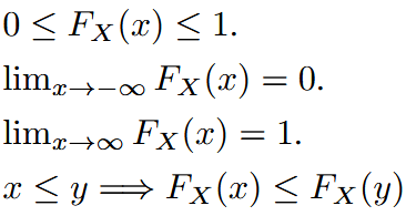
probability mass function (for discrete random variables)	概率质量函数	$p_X(x)=P(X=x)$$p_X(x)=P(X=x)$ properties: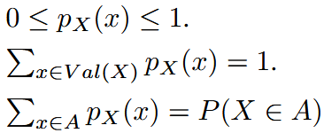
probability density function (for continuous random variable)	概率密度函数	$f_X(x)\triangleq \frac{d{F}_X(x)}{dx}$$f_X(x)\triangleq \frac{dF_X(x)}{dx}$ properties: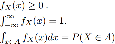
expectation	期望（这里说的是概率期望）	For discrete random variable: For continuous random variable:
		this is kind of “weighted average” of the $g(X)$$g(X)$
		properties:
variance	方差	The variance of a random variable $X$$X$ is a measure of how concentrated the distribution of a random variable $X$$X$ is around its mean $Var[X]\triangleq E[(X-E[X]{)}^2]$$Var[X]\triangleq E[(X-E[X])^2]$ properties: $\begin{array}{c}Var[a]=0\\ Var[af(x)]=a^{2}Var[f(x)]\end{array}$$Var[a]=0\\Var[af(x)]=a^2Var[f(x)]$
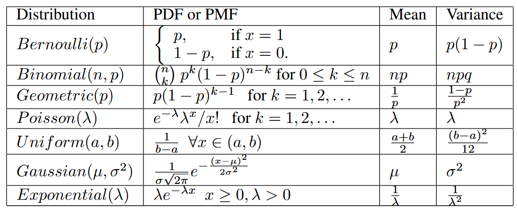
Some common random variables
Bernoulli	伯努利分布
Binomial	二项分布
Geomatric	几何分布
Poisson	泊松分布
Continuous random variables
Uniform	均匀分布
Exponential	指数分布
Normal	正态分布
joint cumulative distribution function	联合累积分布函数	$F_{XY}(x,y)=P(X\le x,Y\le y)$$F_{XY}(x,y)=P(X\le x, Y\le y)$
marginal cumulative distribution function	边缘累积分布函数
joint probability mass function (for discrete random variable )	联合概率质量函数
marginal probability mass function (for discrete random variable )	边缘概率质量函数
joint probability density function	联合概率密度函数
marginal probability density function	边缘概率密度函数
conditional distributions	条件分布
conditional probability density	条件概率密度
bayes’s rule	贝叶斯公式	$P(A|B)=\frac{P(AB)}{P(B)}=\frac{P(B|A)P(A)}{P(B)}$$P(A|B)=\frac{P(AB)}{P(B)}=\frac{P(B|A)P(A)}{P(B)}$
independent	独立（这里说的是多个随机变量）	$F_{XY}(x,y)=F_X(x)F_Y(y)⟶\text{X and Y are independent}$$F_{XY}(x,y)=F_X(x)F_Y(y)\longrightarrow\text{X and Y are independent}$
		if $X$$X$ is independent of $Y$$Y$ then any function of $X$$X$ is independent of any function of $Y$$Y$
expectation and covariance	期望与协方差（多随机变量）
		if $Cov[X,Y]=0,\text{ X and Y are uncorrelated}$$Cov[X,Y]=0,\text{ X and Y are uncorrelated}$
		For more random variables
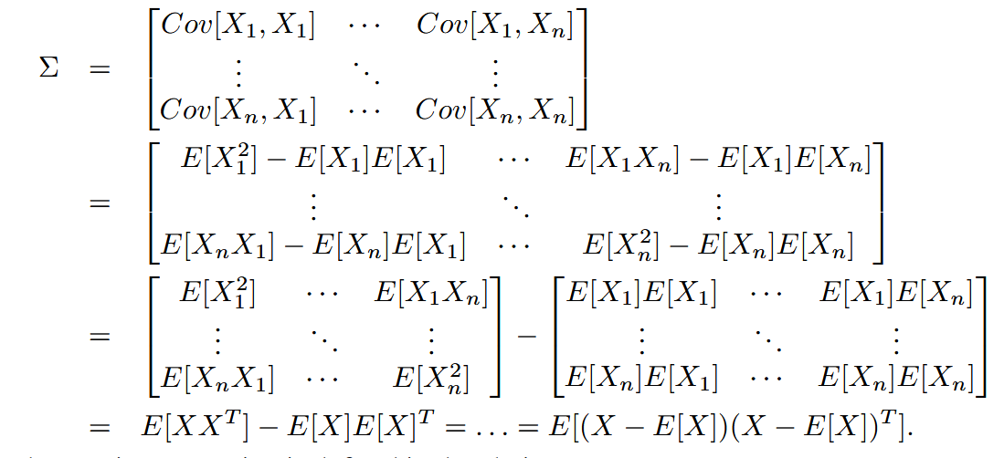		this is for random vector and covariance matrix
rule of total probability	总概率法则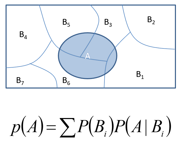

Machine Learning

English	中文	Complementary
gradient descend	梯度下降	$J(\theta )$$J(\theta)$ is the loss function
batch gradient descend	批量梯度下降
		For gradients, the loss function is only one global, and no other local, optima.
stochastic gradient descent (incremental gradient descent)	随机梯度下降（增量梯度下降）SGD	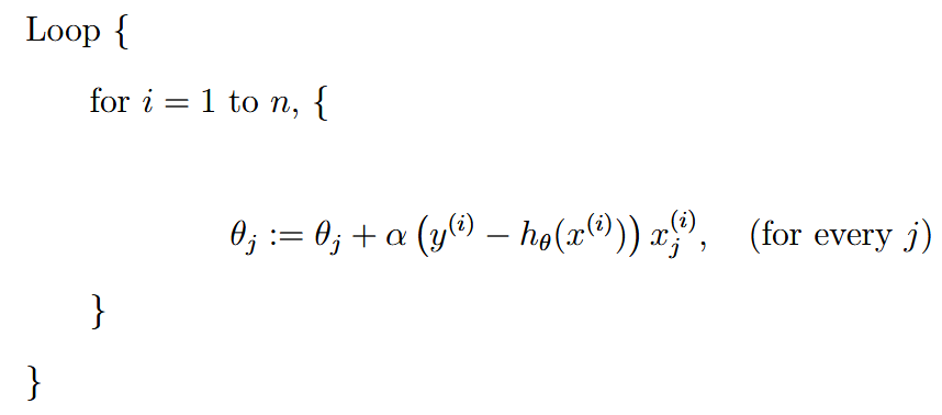一次只看一个，看一个更新一次 Often, stochastic gradient descent gets θ “close” to the minimum much faster than batch gradient descent. 当训练集非常大的时候，SGD每次更新都能看到效果，所以很不错。此时一次性更新一个训练集的批量梯度下降的开销太大
least squares	最小二乘法	前面的梯度下降需要迭代，这里使用最小二乘法直接算出θ的封闭解
independently and identically distributed=	独立同分布
likelihood	似然函数	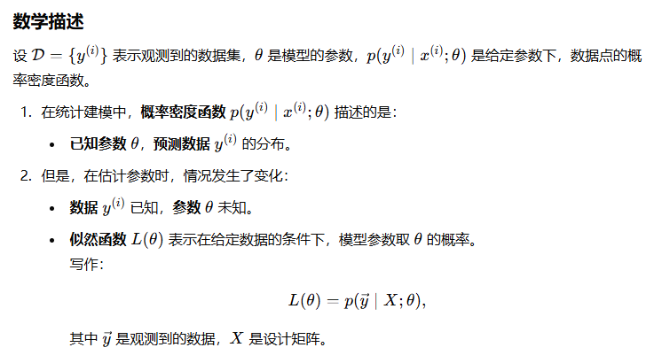就是倒过来，数据集中已知x和y的情况。$\theta$$\theta$的取值使得取这个y最大 说白了就是找到使得p最大的参数θ
maximum likelihood	最大似然	we should choose θ so as to make the data as high probability as possible. I.e., we should choose θ to maximize $L(\theta )$$L(\theta)$. 为了方便计算，一般会使用对数似然函数，就是说白了取个log
sigmoid function / logistic function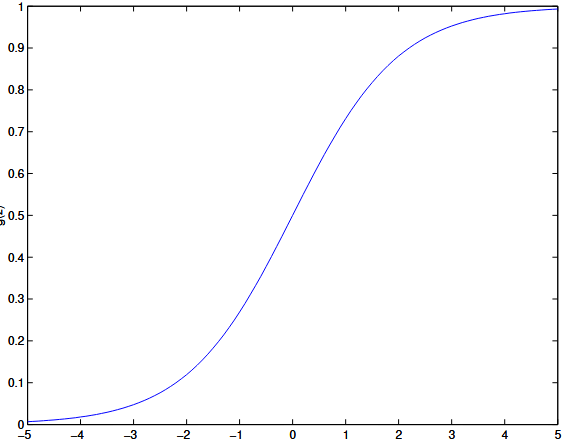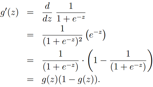
regression	回归
multinominal distribution	多项分布
softmax	归一化操作	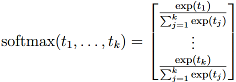We usually call the $t_i$$t_i$ here as “logits”
Newton’s method	牛顿法	也是一个优化方法 找0点 通过寻找二阶导的零点来找寻梯度为0的点，进而寻找极值进行优化（找最大值需要让hessian矩阵为正，也就是二阶导或者说曲率为正，反之相反) 详见pdf
generalized linear models	广义线性模型（GLM）
exponential family	指数族	如果能被写成这个形式，那么一个分布就可以被划为指数族 详见pdf
discriminative learning algorithms	判别式学习算法	求$P(y|x)$$P(y|x)$，也就是知道输入，直接输出y
generative learning algorithms	生成式学习算法	建模学习$P(x|y)$$P(x|y)$，也就是学习已知类别的特征，然后使用贝叶斯或者别的算法来算最后的输出
class priors	类先验	类先验p(y)是指在没有任何观测数据x的情况下，某一类别y出现的概率。 （利用贝叶斯来计算最后的值） 这里$p(y)$$p(y)$式是类先验。这里有几个y就可以带入几次来看最后的概率 这里$p(x)=p(x|y=1)p(y=1)+p(x|y=0)p(x=0)$$p(x)=p(x|y=1)p(y=1)+p(x|y=0)p(x=0)$（实际计算中不需要计算这个，因为这个是分母，我们找寻的是取最大值时的y，分母不影响)
multivariate normal distribution	多随机变量正态分布
gaussian discriminant analysis (GDA)	高斯判别分析	详见pdf 4.1.2 基本就是一个multivariable normal distribution的generative learning algorithm
		GDA makes stronger modeling assumptions, and is more data efficient (i.e., requires less training data to learn “well”) when the modeling assumptions are correct or at least approximately correct. Logistic regression makes weaker assumptions, and is significantly more robust to deviations from modeling assumptions GDA有着更强的假设，也就意味着更弱普适性 GDA数据效率更高，但是适合的数据类型少，实际应用中逻辑回归更为常见
Naive Bayes (NB) assumption	朴素贝叶斯假设	计算$P(x|y)$$P(x|y)$的时候如果x过于大了，比如x是一个5000维的向量，那么就有$2^{5000}-1$$2^{5000}-1$个参数（这里是因为4999个参数能够确认49999个概率，概率和为1，所以第5000个自然可以知道）。 这个时候就需要假设：$x_i$$x_i$‘s are conditional independent given y （x直接互相独立） 记住是在given y的情况下，也就是说 并不一定成立
Naive Bayes classifier	朴素贝叶斯分类器
discretize	离散化	convert continuous variables to discrete variables (usually when using naive bayes to continuous variables)
laplace smoothing	拉普拉斯平滑	Sometimes the input may never appearing the training set, which will cause all the result to 0 or 0/0 like: To mitigate it: $⟹$$\Longrightarrow$
numerator	分子
denominator	分母	拉普拉斯平滑分母上加的k通常是所有样本数目，因为必须要保证概率和为1
cubic function	三次函数
RHS	右边	right hand side
kernel trick	核技巧	通过换元避免在高维空间中进行大量的计算（详见pdf 5.3）
		kernel的最后一节最后完全没看懂 重新看一遍
support machine learning	支持向量机
separating hyperplane	分离超平面	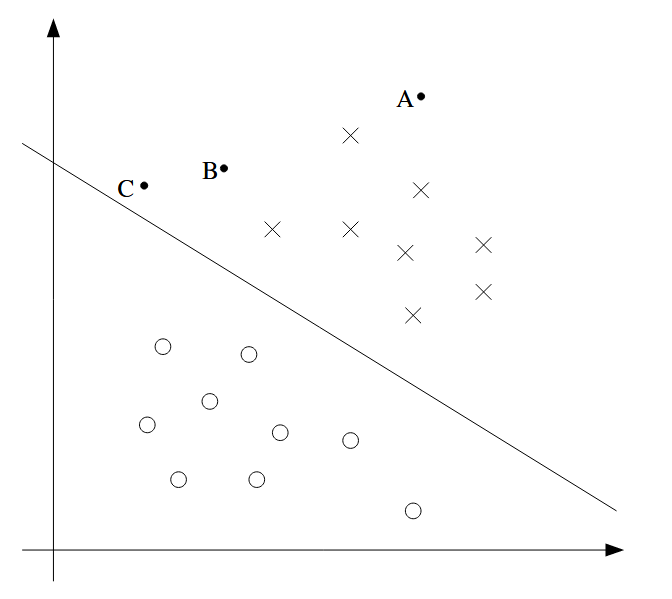图中斜线
margin	边距	离”separating hyperplane“的“距离”，一般而言点离这个分界线越远，对于该点的预测更加confident
functional margin	功能边距	该值为正的时候预测正确（负负或者正正)，为负的时候错误（一正一负)。同样希望这个距离很大，这样更加confident
geometric margin	几何边距	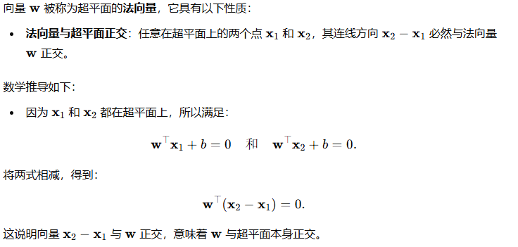$y=w^{T}x+b,w$$y=w^Tx+b,w$始终垂直于separating hyperplane 具体推导看63页
		把这个边距$\gamma$$\gamma$理解为置信度就很轻松了（我们需要最大化最小将e）
lagrange duality	拉格朗日对偶性
activation function	激活函数	Typically, for multi-layer neural network, at the end, near the output, we don’t apply ReLU (or other activation functions), especially when the output is not necessarily a positive number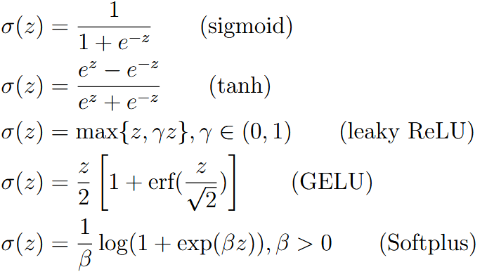 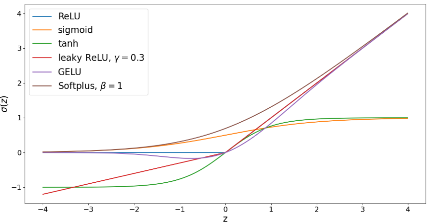NOTE: the $tanh$$tanh$ and $sigmoid$$sigmoid$ are used less and less because the gradient of them vanishes as the value goes both positive and negative infinity.
relu	某种激活函数	$ReLU(t)\triangleq max\{t,0\}$$ReLU(t)\triangleq max\{t,0\}$
vectorization	向量化	如果一个neural network里面每次参数与x计算都单独算的话，会大量地使用for循环。这样计算效率会非常低。所以使用线性代数来进行向量化，加快并行计算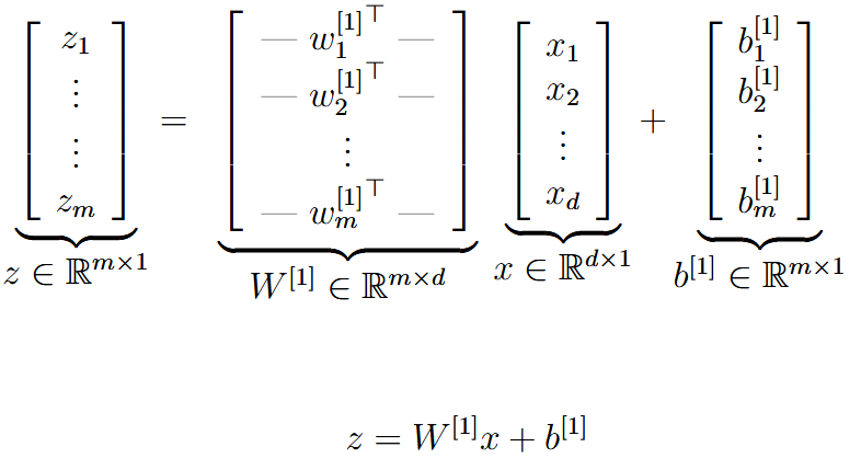
identity function	恒等函数	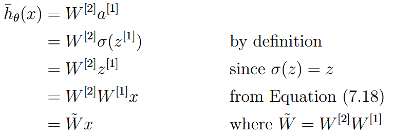$e.g.y=x$$e.g. \ y=x$ We do not use identity function as the activation function because we wanna introduce non-linear instead of: (apply a linear function to another linear function will also end to a new linear function)
feature engineering	特征工程	the process of designing the feature maps $\varphi (x)$$\phi(x)$ We can view deep learning as a way to automatically learn the right feature map (sometimes also referred to as “the representation”) 神经网络通常不用人们像传统的特征工程里面去精心根据领域知识（domain knowledge）去设计特征映射，每一个神经元可以自己学习
multi-layer perceptron	MLP
residual connection	残差连接
layer normalization (LN)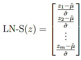
		这里求解deviation的时候除的m而不是m-1，是因为想让LN输出的和为1
		Oftentimes zero mean and standard deviation 1 is not the most desired normalization scheme
scaling-invariant property	放缩不变性
		when we talk about the weights’ scaling-invariant property, we usually talk about the weights except the last layer. Because usually we do not do normalization to the last layer (same as the activation function)
		Batch normalization and group normalization are more often used in computer vision applications whereas layer norm is used more often in language applications.
convolutional layers	卷积层	For one dimension: $Conv1D-S(x)$$Conv1D-S(x)$, the parameters are a filter vector (kernel) $w\in {\mathbb{R}}^k$$w\in \mathbb{R}^k$, where the k is filter size. We assume the $k=2\ell +1$$k=2\ell+1$, is odd 对于超出原始z的值，padding为0 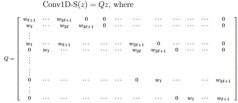multiple channel version:
		一维卷积往往用于NLP领域，二维卷积往往用于视觉处理
backpropagation	反向传播
partial derivatives	偏导
chain rule	链式法则	background: 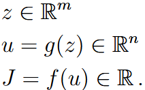chain rule (for scalars and vectors): 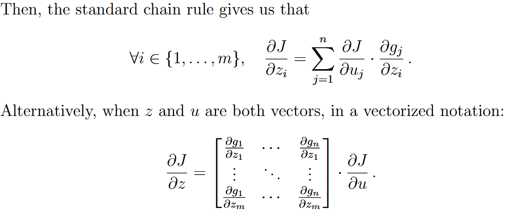for simplicity:
		Backpropagation contains two stages: forward pass and backward pass. During the forward pass, it will save all the intermediate variables
generalization	泛化性
overfit	过拟合	the model perform well on training set but not that good on test set
underfit	欠拟合	the model perform not good even training set
bias-variance tradeoff	偏差-方差权衡
bias	偏差	the bias captures the part of the error that are introduced due to the lack of expressivity of the model 很多时候是模型不够强大导致，比如使用一次函数预测二次函数生成的数据集。也可能是数据集不够。总而言之就是欠拟合
variance	方差	The variance term captures how the random nature of the finite dataset introduces errors in the learned model (It measures the sensitivity of the learned model to the randomness in the dataset. It often decreases as the size of the dataset increases.) 可能是因为模型过于强大（数据量不足会加剧这个），导致其捕捉了很多无关信息，比如数据生成过程的噪声。说白了就是过拟合
		Often, there is a tradeoff between bias and variance. If our model is too “simple” and has very few parameters, then it may have large bias (but small variance), and it typically may suffer from underfittng. If it is too “complex” and has very many parameters, then it may suffer from large variance (but have smaller bias), and thus overfitting.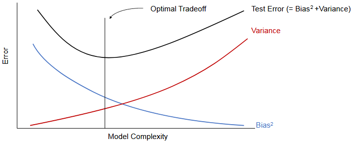 数学推导看pdf121页
double descent phenomenon	双下降现象	模型的error分为两部分，bias和variance，一般而言，随着模型参数量增加，error会呈现出一个先下降后增加的趋势（convex）。然而有时候会下降两次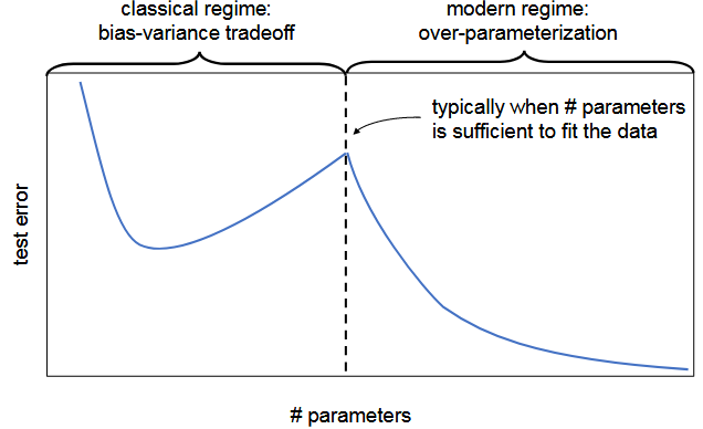 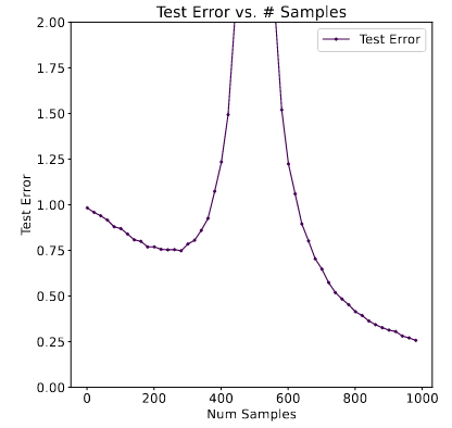对于训练数据同理。图一model-wise，图二sample-wise
		To some extent, sample-wise double descent and model-wise double descent are essentially describing similar phenomena—the test error is peaked when n ≈ d.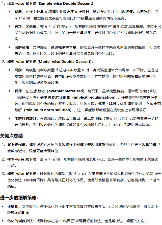
regularization	正则化	$J_{\lambda }=J(\theta )+\lambda R(\theta )$$J_\lambda=J(\theta)+\lambda R(\theta)$, $\lambda$$\lambda$ is the regularization parameter the regularizer $R(\theta )$$R(\theta)$ (e.g. ${\ell }_2$$\ell_2$ norm) is typically chosen to be some measure of the complexity of the model $\theta$$\theta$
weight decay	权重衰减（欧几里得范数正则）
		$\begin{array}{c}\parallel \theta {\parallel }_1=\sum _i|{\theta }_i|\\ \frac{1}{2}\parallel \theta {\parallel }_2^2=\frac{1}{2}\sum _i{\theta }_i^2\end{array}$$\|\theta\|_1=\sum_{i}|\theta_i|\\\frac{1}{2}\|\theta\|_2^2=\frac{1}{2}\sum_i\theta_i^2$
implicit regularization effect	隐式正则化效果	optimizers can implicitly impose structures on parameters beyond what has been imposed by the regularized loss 正则化的训练loss也许不止一个全局最优解，即使在训练集上同样效果，但是有的优化器可能会因为将模型变得更加稀疏或怎样，使得其在测试集上效果更好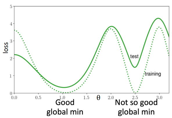
		In summary, the takehome message here is that the choice of optimizer does not only affect minimizing the training loss, but also imposes implicit regularization and affects the generalization of the model. Even if your current optimizer already converges to a small training error perfectly, you may still need to tune your optimizer for a better generalization.
Lipschitz		more Lipschitz model: 更平滑的模型，模型在输入空间中对输入变化的响应更为平缓或稳定。
cross validation	交叉验证	说白了就是把数据分成训练集和测试集，在训练集上训练，然后选择测试集上误差最小的模型。
k-fold cross validaition	k折交叉验证	普通交叉验证要浪费一部分数据，因为测试集不能用于训练。 K折：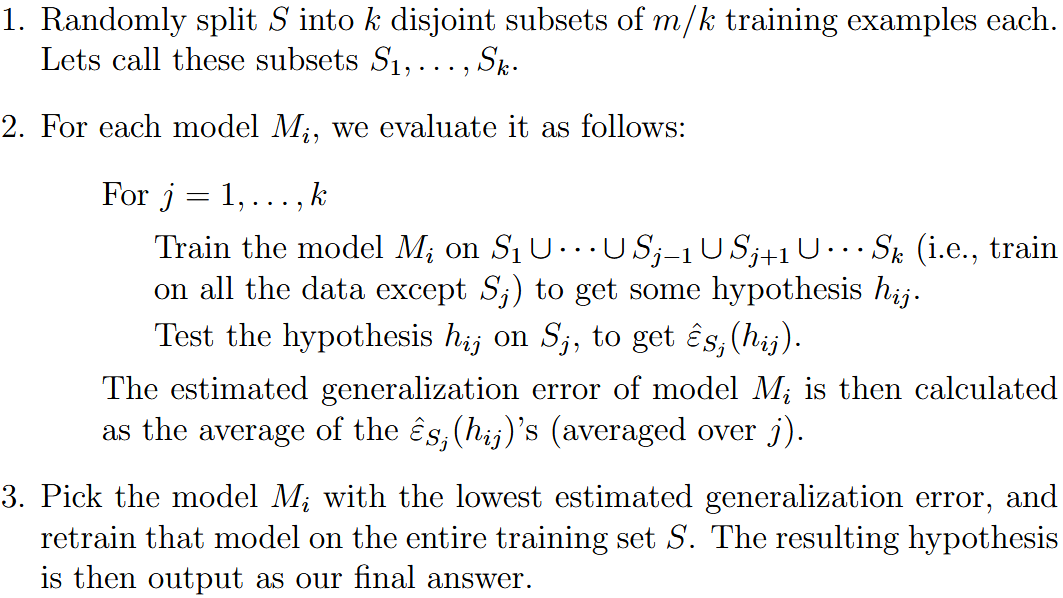
leave-one-out cross validation	留一法交叉验证	数据实在太少的时候，k就等于数据量。每次只留一个数据
maximum likelihood estimation (MLE)	最大似然估计
		this is used to estimate the parameter $\theta$$\theta$
clustering	聚类	只有x没有y，是一种unsupervised learning problem n the clustering problem, we are given a training set {x(1), . . . , x(n)}, and want to group the data into a few cohesive “clusters.”
k-means	k近邻	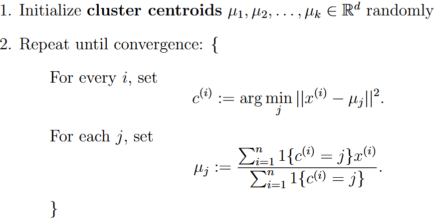先随机选k个中心点。根据距离聚类，每一类产生一个新的中心点，直到收敛。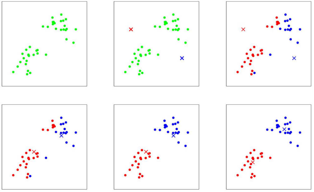
distortion function	畸变函数	J的值随着kmeans的循环是单调递减的，所以kmeans一定收敛 但是kmeans也有可能只是局部最佳，可以多次运行更换初始值避免
Mixture of Gaussians	混合高斯模型	background: 就是说我们只能观测到x，但是x是由隐变量z决定的正态分布产生的 每个x对应一个隐藏的不可观测的z所对应的高斯分布，所以是混合高斯模型
latent random variable	隐变量	隐变量z决定了生成x的高斯分布，如果我们知道z是什么，那么上面的似然估计就可以写成： 这里的优化问题就和gaussian discriminant analysis很像了，这里的z就像是GDA里面的y。 但是！不一样的是！我们这里并不知道z！
evidence lower bound	ELBO
EM algorithm (expectation-maximization)	期望最大化算法	分为E和M两步，E步的时候就直接猜z的值，M步的时候就要假装E猜的是对的，然后进行优化 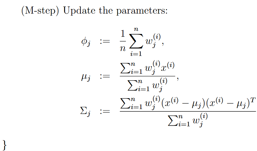（这里E的时候也不是乱猜的，是使用的贝叶斯去算的z的后验概率，然后把这个后验概率假装是正确的）
		EM和kmeans其实很相似。不同之处在于kmeans在初始化（可以看作第一个E步的时候）使用hard guess，直接随机初始化了几个点。而EM在E的时候（*这里）使用的是soft guess。 EM同样会有可能遭遇到局部最优的情况
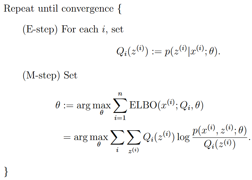		使用z关于x的后验概率当作z的分布（soft guess）（推导见：pdf 11.3） 这里其实就是下界优化，最大化ELBO
Jensen’s inequality	詹森不等式	如果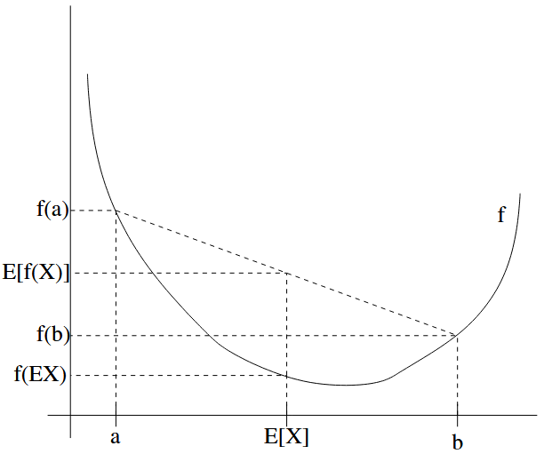$f(x)$$f(x)$是严格convex（凸函数，向下凹），那么有$E[f(x)]\ge f(E[x])$$E[f(x)]\ge f(E[x])$，当$X=E[X]\text{ with probability }1$$X=E[X]\text{ with probability }1$ 如果这个函数的hessian矩阵式半正定 (positive semi-definite)，那么他是凸函数，如果是正定的，那么是严格凸函数 对于凹函数同样适用，把符号改个方向就好了
concave/convex function	凹函数/凸函数	这里的理解和中文语境里面的凹凸其实是相反的
variational inference	变分推理	在EM算法中，我们是有posterior probability p(z|x, θ)，来当作z的概率，但是实际情况中这个可能会十分难以计算。所有变分推理中寻找approximation of the true posterior distribution 在一个分布族$\mathcal{Q}$$\mathcal{Q}$里面找到最大化下界ELBO的
mean filed assumption	平均场假设	对于高维discrete random variable z来说，使用平均场假设
		mean filed assumption仅仅针对于离散的，对于continuous random variable而言 q v分别是两个函数
re-parameterization	重参数化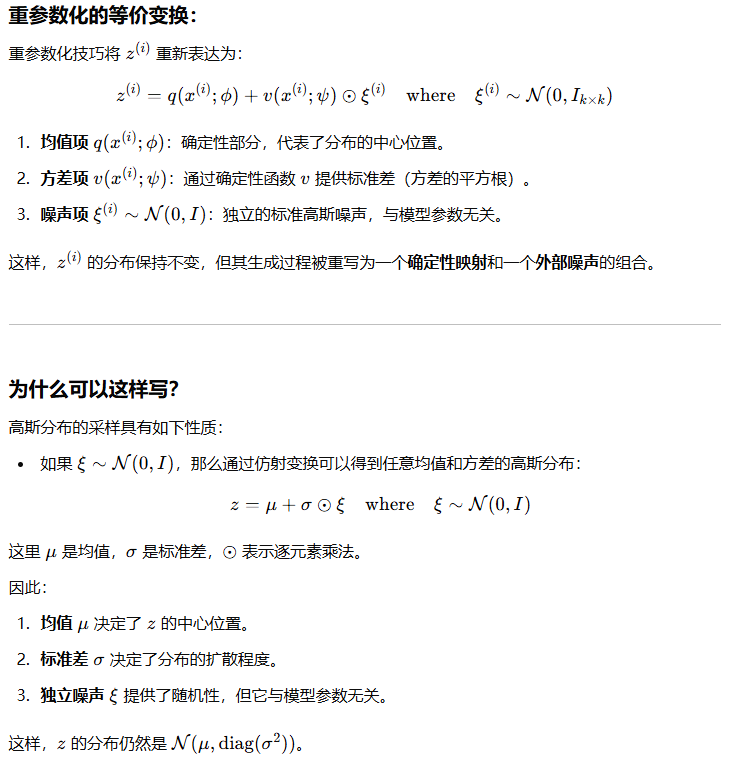
		变分推导和变分自编码器看pdf 13.5，目前没太看懂 大概意思是使用一个Q的估计，因为Q太难算了。但是这个估计的形式我没看懂
principal components analysis (PCA)	主成分分析	数据压缩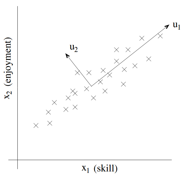 to find the major axis of variation $u_1$$u_1$
		Before PCA, first normalize the data by $\begin{array}{c}{x}_j^{(i)}\leftarrow \frac{x_j^{(i)}-{\mu }_j}{{\sigma }_j}\\ {\mu }_j=\frac{1}{n}\sum _{i=1}^n{x}_j^{(i)}\text{and}{\sigma }_j^2=\frac{1}{n}\sum _{i=1}^n(x_j^{(i)}-{\mu }_j{)}^2\end{array}$$x_j^{(i)} \leftarrow \frac{x_j^{(i)} - \mu_j}{\sigma_j}\\\mu_j = \frac{1}{n} \sum_{i=1}^{n} x_j^{(i)} \quad \text{and} \quad \sigma_j^2 = \frac{1}{n} \sum_{i=1}^{n} (x_j^{(i)} - \mu_j)^2$. ensures that different attributes are all treated on the same “scale.” Make different attribute more comparable
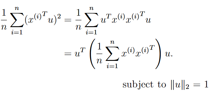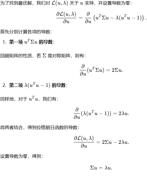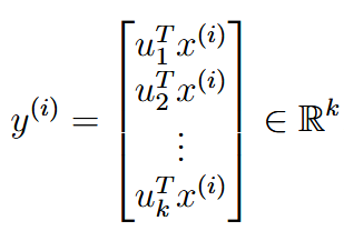independent components analysis (ICA)	独立成分分析	background: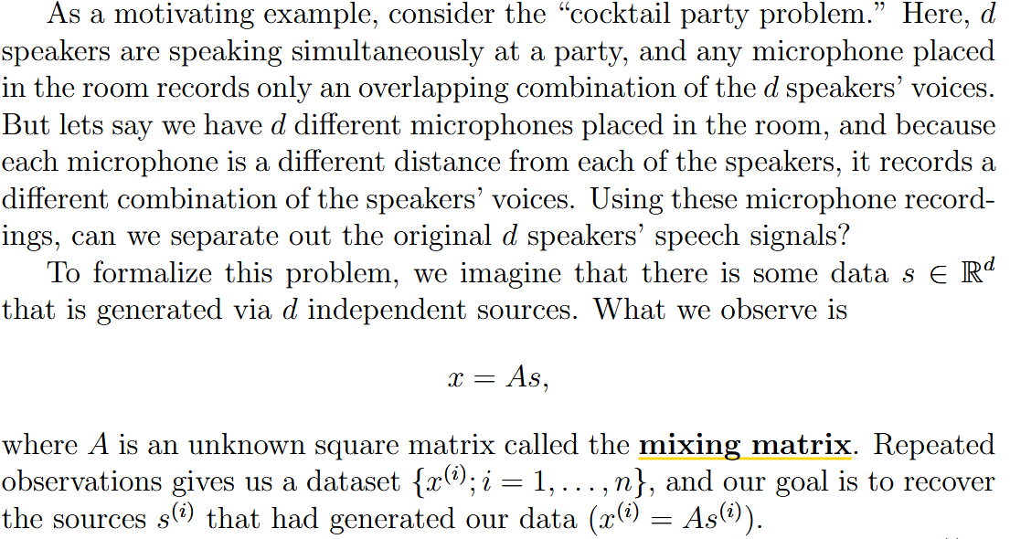 这里s是说话的人，A是混合，x是最后录入的结果，目标是复原s，也就是找到$W=A^{-1}$$W=A^{-1}$
permutation matrix	排序矩阵	如： 每一行每一列有且仅有一个1
ICA ambiguities	ICA 模糊性	pdf 13.1 大概意思就是对W的scale很多情况下不影响，即使还原的s会不同，比如放缩或者正负。但是放缩这些对于声音数据来说就是调节了一下音量。很多别的应用场景这个同样不影响
		高斯分布的旋转对称性导致无法通过 ICA 恢复原始独立源，但只要数据源是非高斯分布，就可以消除这种不确定性，从而唯一确定独立源。
		ICA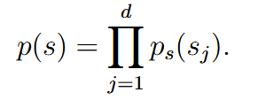： 这里指定z的CDF是sigmoid，这个可以自己选择，只要不是高斯分布就行
reinforcement learning	强化学习	In the reinforcement learning framework, we will instead provide our algorithms only a reward function, which indicates to the learning agent when it is doing well, and when it is doing poorly.
markov decision process (MDP)	马尔可夫决策过程	$\begin{array}{c}State:\text{状态}\\ Action:\text{行为}\\ \gamma :\text{discount factor 折扣因子}\\ Reward:\text{奖励函数 }R\in {\mathbb{R}}^{S\times A}\end{array}$$State: \text{状态} \\Action: \text{行为} \\\gamma: \text{discount factor 折扣因子} \\Reward :\text{奖励函数 }R\in \mathbb{R}^{S\times A}$
		最终优化目标：最大化奖励和的期望值
policy	决策	$\begin{array}{c}\pi :S\to A\\ a=\pi s\\ \text{value function}:\end{array}$$\pi \ : \ S\rightarrow A\\a=\pi s \\\text{value function}:$
Bellman equations	贝尔曼等式	如果policy $\pi$$\pi$ 固定， 这里是一个recursive function，第一个是intermediate reward，是初始阶段获得的奖励，后面就是一个递归（后面这项其实是一个期望，就是p(x) * ) 这个贝尔曼等式用于解决有限状态（要求决策固定)的时候十分好用
value iteration	价值迭代	（有限状态与action) synchronous update：每次一个loop之后再全部更新 asynchronous update：每次一个V都更新，异步
policy iteration	策略迭代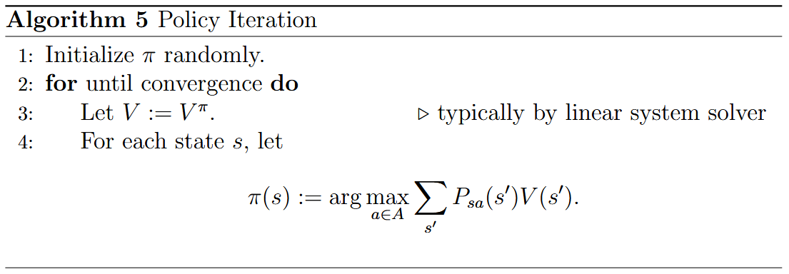
		learning the MDP
Continuous state MDPs	连续状态马尔科夫决策过程	上面都的情况state都是discrete，现在讨论连续的，意思就是state就infinite个
discretization	离散化	用一些离散值来表示一个连续值 有两个缺点： 1. 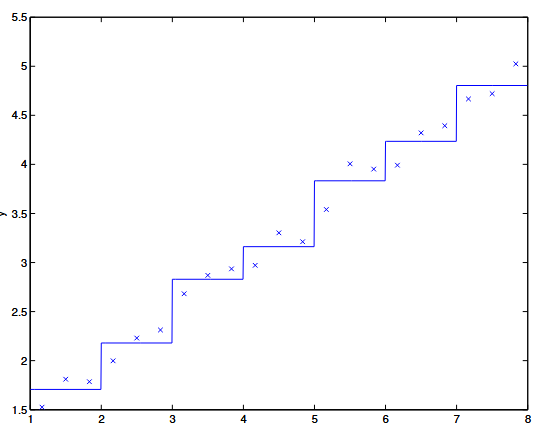并不够平滑 2. curse of dimensionality 维度诅咒。For example, for $S\in {\mathbb{R}}^d$$S\in \mathbb{R}^d$, for each of the d dimension, if we discretize it into k values, then there will be $d^k$$d^k$ states. if d is 1000 and k is 10, then the value is very huge. (so discretization is usually used for low dimensions like 2- 6)
value function approximation	值函数近似	近似这个函数
		we assume we have a model, or simulator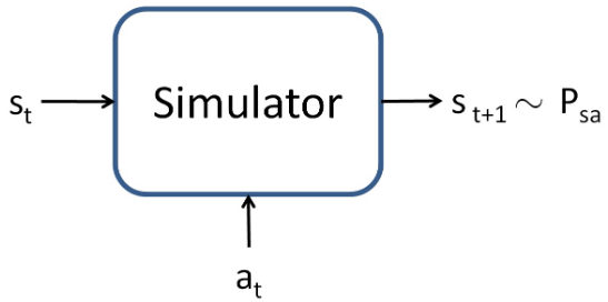 这个simulator可以有多种形式。比如使用物理模拟器、多跑几个trial得到distribution计算，或者就是自定义一个模型（神经网balalala)
Fitted value iteration	拟合值迭代	假设state连续，但是action很少并且离散 For continuous state: （就是从state空间里面取样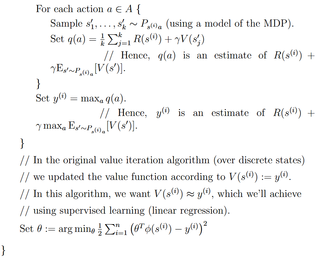） 这里也是采样k个，因为是连续的有无数个，所以只采样k个进行近似
finite horizon MDP	有限视野MDP	取消了discount factor，加入了time factor。 And this is general for both discrete and concrete states and actions