Course Homepage: 15-462/662 Fall 2020
For assignments implementations: tbbbk/Scotty3D_Benky
Author: Bingkui Tong
1. Basic Math Review1.1 Linear Algebra Review1.1.1 Norm1.1.2 Linear Map1.1.3 Gram-Schmidt1.2 Vector Calculus1.2.1 Matrix Representation of Cross Product1.2.2 Determinant of a Linear Map1.2.3 Derivative as Best Linear Approximation1.2.3 Gradients of Matrix-Valued Expressions1.2.4 Vector Fields1.2.5 Divergence 散度1.2.6 Curl 旋度1.2.7 Hessian in Coordinates2. Rasterization2.1 Rasterization 101: Drawing a Triangle2.1.1 Pinhole camera2.1.2 Computing triangle coverage2.1.3 Aliasing2.1.4 SuperSampling2.2 Spatial Transformations2.2.1 Rotation2.2.2 Scaling2.2.3 Shear2.2.4 Composition2.2.5 Polar & Singular Value Decomposition2.2.6 Interpolating Transformations—Polar2.2.7 Translation!2.2.8 Homogeneous Coordinates2.2.9 Transformation Composition Order2.2.10 Scene Graph2.3 3D Rotations and Complex Representations2.3.1 Degree of Freedom2.3.2 Commutativity of Rotation—3D2.3.3 Euler Angles—Gimbal Lock2.3.4 Complex Analysis2.3.5 Rotation: Matrices vs.Complex2.3.6 Quaternions 四元数2.3.7 3D Rotations via Quaternions2.4 Perspective Projection2.4.1 View Frustum2.4.2 Clipping2.4.3 Mapping Frustum to Unit Cube2.5 Texture Mapping2.5.1 Barycentric Coordinates2.5.2 Perspective Correct Interpolation2.5.3 Texture Coordinates2.5.4 Magnification vs. Minification2.5.5 Bilinear Interpolation (Magnification)2.5.6 MIP Map (Minification)2.5.7 Trilinear Interpolation for MIP Map2.5.8 Anisotropic Filtering2.6 Depth and Transparency2.6.1 Depth-Buffer2.6.2 Compositing2.6.3 Fringing2.6.4 (Non-) Premultiplied Alpha2.7 Rasterization Pipeline Summary3. Geometry3.1 Encode Geometry3.1.1 Implicit Representations3.1.2 Explicit Representations3.1.3 Summary3.2 Meshes and Manifolds3.2.1 Manifold Assumption3.2.2 Why Do We Need Manifold?3.2.3 Halfedge Data Structure3.2.4 Halfedge Meshes Edition3.3 Digital Geometry Processing3.3.1 Remeshing as Resampling3.3.2 Upsampling via (Catmull-Clark/Loop) Subdivision3.3.3 Simplification via Edge Collapse3.3.4 Isotropic Remeshing Algorithm3.5 Geometric Queries3.5.1 Ray Equation3.5.2 Intersection3.6 Spatial Acceleration Data Structures3.6.1 Affine Map for Triangle3.6.2 Bounding Box3.6.3 Bounding Volume Hierarchy (BVH)4. Ray Tracing4.1 Color4.1.1 Intensity or Absorption4.1.2 Emission and Reflection4.1.3 Color Models4.1.4 Y’CbCr4.2 Radiometry4.2.1 Photon4.2.2 Radiant Energy
1. Basic Math Review
I didn't write everything in detail for this section.
1.1 Linear Algebra Review
1.1.1 Norm
Which measures total size, length, volume, intensity, etc.
Warning: L2 Norm does not encode geometric length unless vectors are encoded in an orthonormal basis.
1.1.2 Linear Map
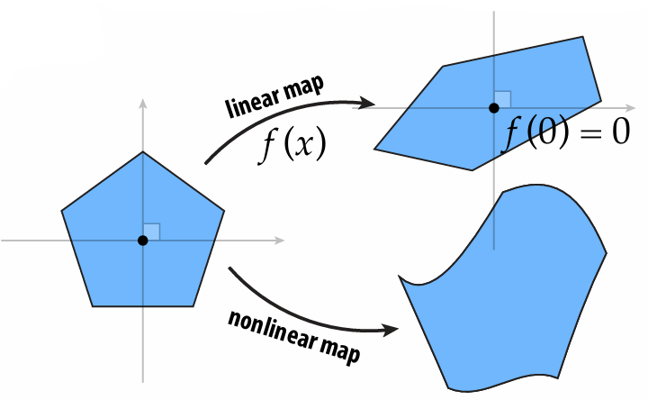
Key Idea: linear maps take lines to lines while keeps the origin fixed
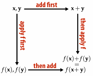
It doesn't matter whether we add the vectors or apply the linear map first.
1.1.3 Gram-Schmidt

Warning: for large number of vectors / nearly parallel vectors, this is not the best algorithm
1.2 Vector Calculus
1.2.1 Matrix Representation of Cross Product
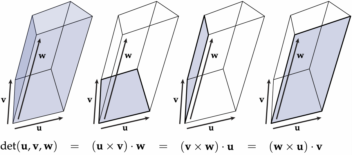
1.2.2 Determinant of a Linear Map
1.2.3 Derivative as Best Linear Approximation
Taylor series:
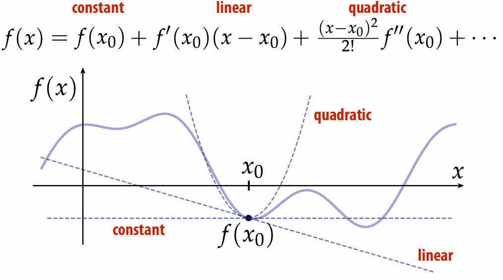
Replacing complicated functions with a linear (and sometimes quadratic) approximation is a powerful trick in graphics algorithms.
1.2.3 Gradients of Matrix-Valued Expressions
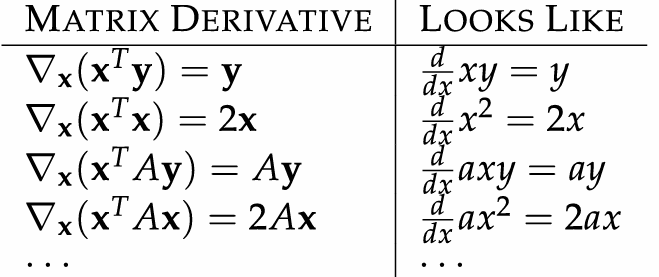
resource: matrixcookbook.pdf
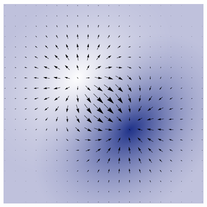
1.2.4 Vector Fields
In general, a vector filed assigns a vector to each point in space, for example, we saw a gradient field:
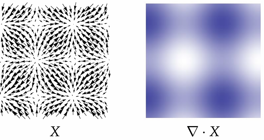
1.2.5 Divergence 散度
Commonly written as
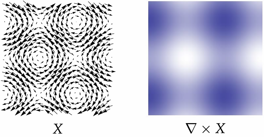
1.2.6 Curl 旋度
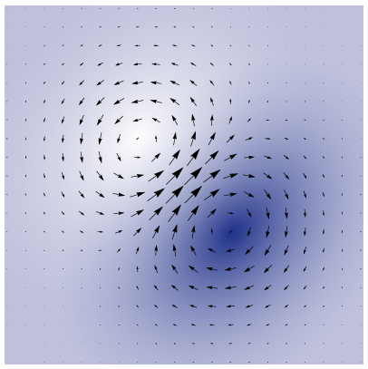
Commonly written as
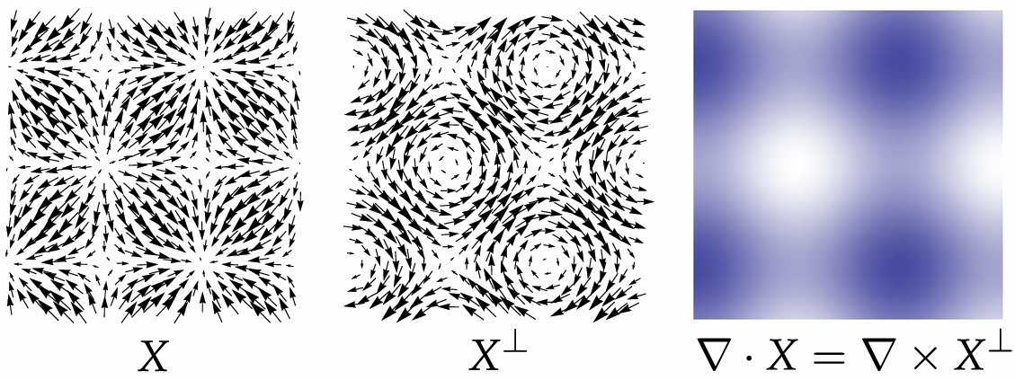
Divergence of
is the same as curl of 90-degree rotation of
1.2.7 Hessian in Coordinates
Hessian is operator that gives us partial derivatives of the gradient.
2. Rasterization
2.1 Rasterization 101: Drawing a Triangle

Why triangle?
Can approximate any shape
always planar, well-defined normal
easy to interpolate data at corners
barycentric coordinates
Key reason: once everything is reduced to triangles, can focus on making an extremely well-optimized pipeline for drawing them
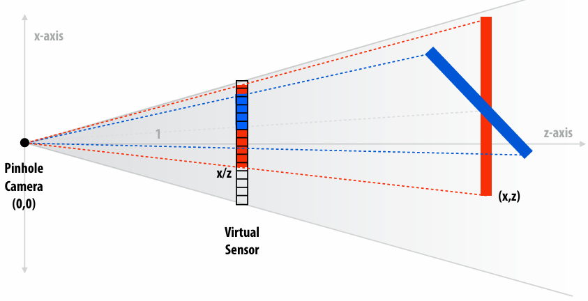
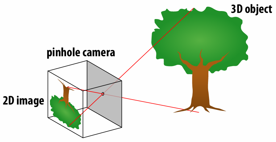
2.1.1 Pinhole camera
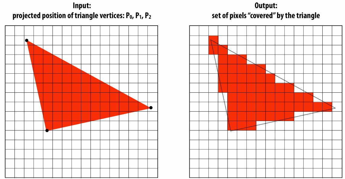
2.1.2 Computing triangle coverage
Key question: Which pixels does the triangle overlap?
2.1.3 Aliasing
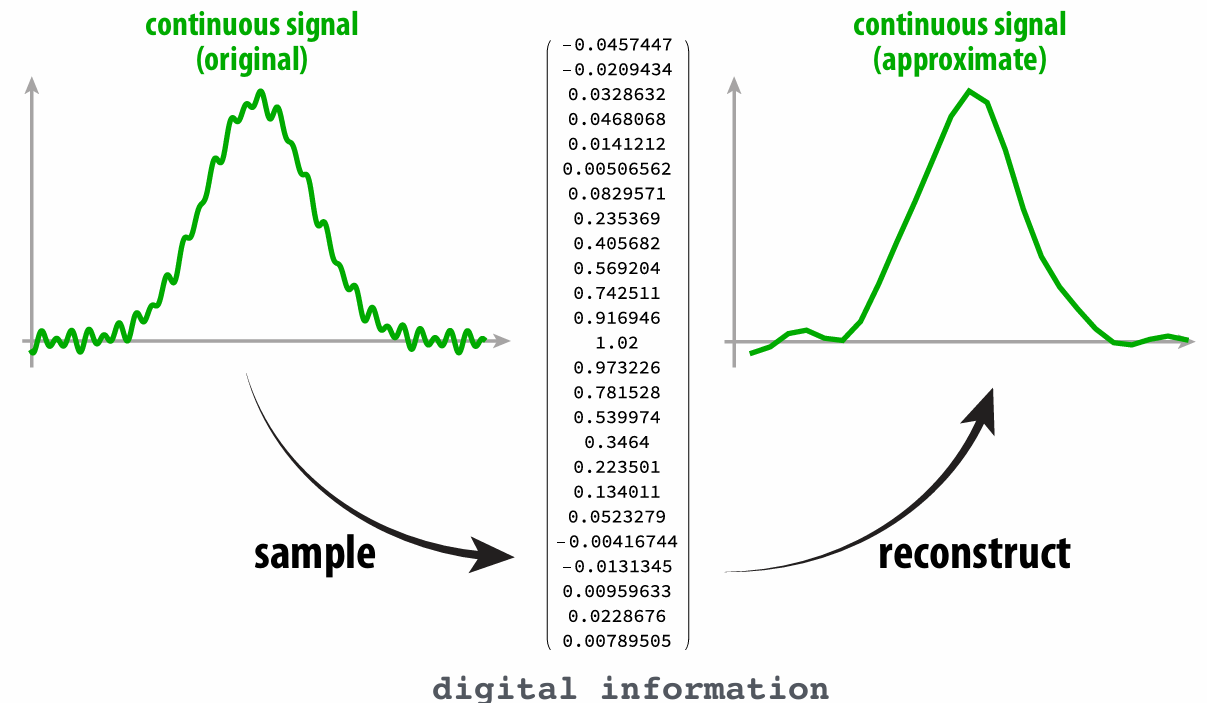
The sampling process lose some information, leading the reconstruction result not exactly accurate. Or we say undersampling high-frequency signals results in aliasing.
2.1.4 SuperSampling
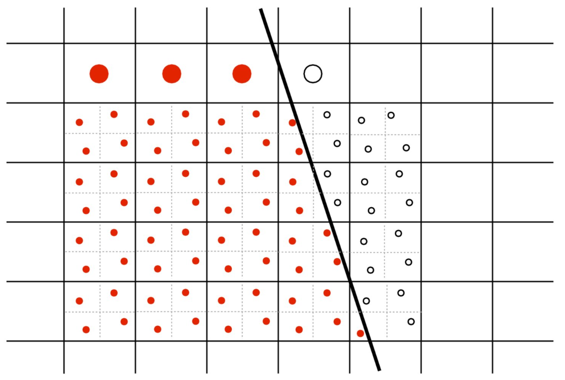
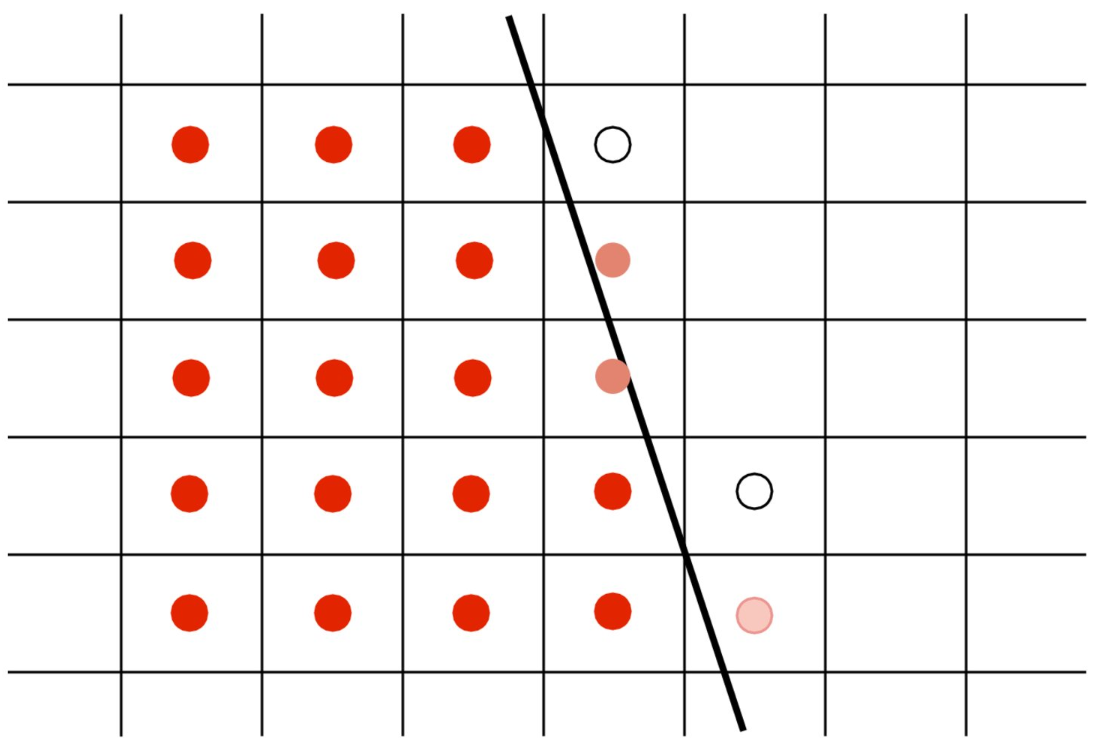
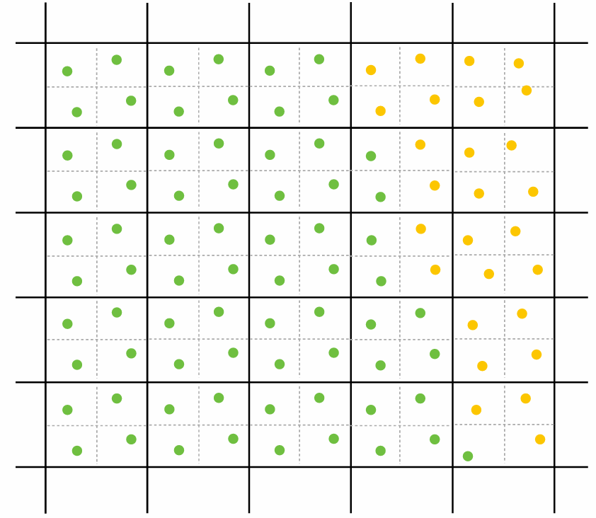
Split a pixel into
2.2 Spatial Transformations
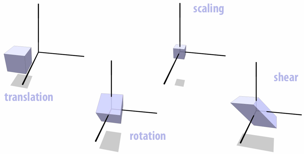
2.2.1 Rotation
Properties:
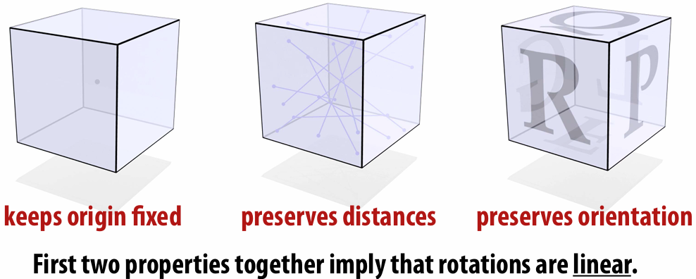
Matrix Representations:
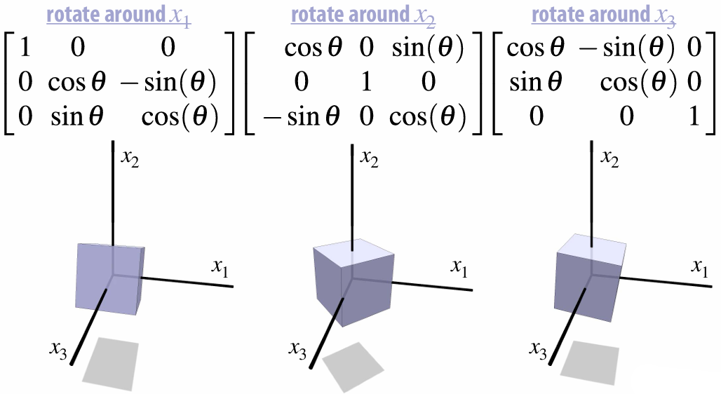
For rotation matrix, the transpose matrix equals inverse matrix.
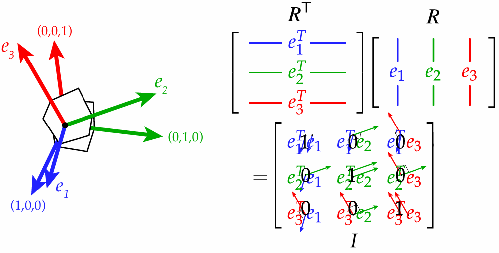
Orthogonal Transformations
We said the rotation inverse matrix equals transpose matrix, but not all
does not mean it is a rotation. When
,
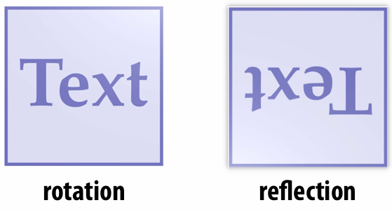
Rotations additionally preserve orientation:
Reflections reverse orientation:
2.2.2 Scaling
Matrix Representations:
Spectral Theorem:
A symmetric matrix
has
orthonormal eigenvectors
real eigenvalues
Hence, every symmetric matrix performs a non-uniform scaling along some set of orthogonal axes.
If
is positive definite ( ), this scaling is positive
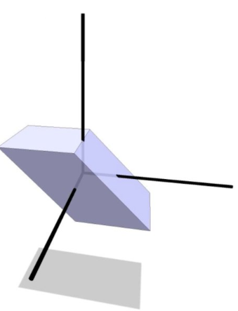
2.2.3 Shear
2.2.4 Composition
We can composite transformations:
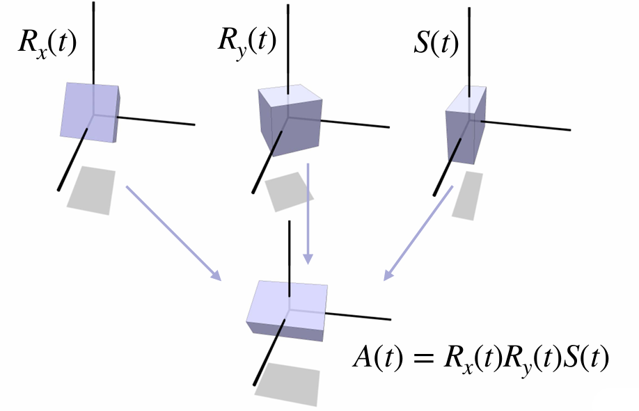
How do we decompose a linear transformation into pieces?
2.2.5 Polar & Singular Value Decomposition
Polar decomposition decomposes any matrix
Since
Where
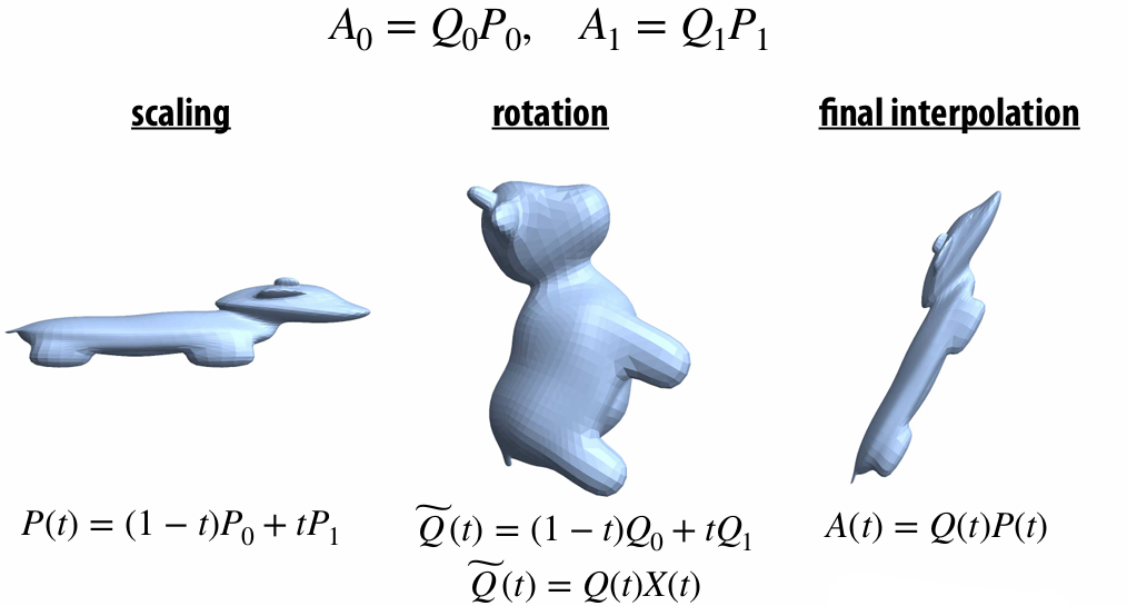
2.2.6 Interpolating Transformations—Polar
2.2.7 Translation!
This transformation is NOT linear!
Additivity
Homogeneity
Translation is AFFINE, not linear. Hence we cannot composite it with other linear transformations.
So, how do we composite all the transformations?
2.2.8 Homogeneous Coordinates
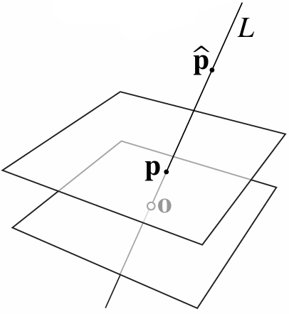
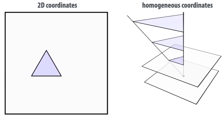
Hint: Every points along a ray represents the same point.
Consider a point
If we apply a translation to a 2D point
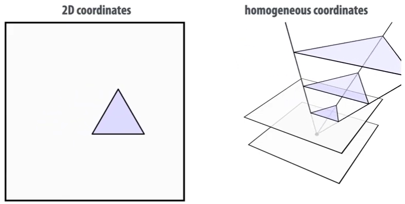
But shear is a linear transformation!
Let a point
Notice that we’re shifting
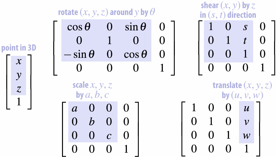
Homogeneous coordinates can also used to distinguish the vectors and points
For vector, the homogeneous coordinate is
, for point the homogeneous coordinate is . Because we cannot translate a vector! So we need to set homogeneous coordinate to to ignore the translation.
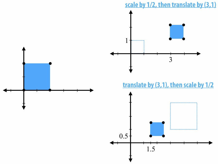
2.2.9 Transformation Composition Order
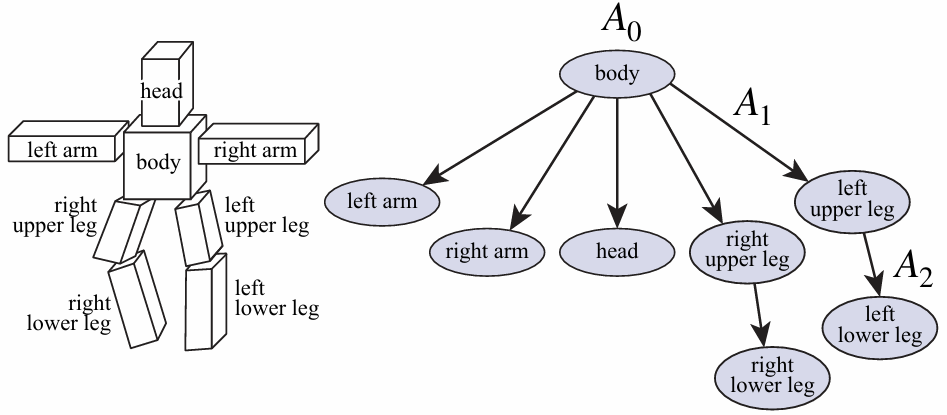
2.2.10 Scene Graph
2.3 3D Rotations and Complex Representations
2.3.1 Degree of Freedom
We need three degrees of freedom to specify a rotation in 3D
Two determine the "axis" direction and one determine how much spinning around the "axis".
2.3.2 Commutativity of Rotation—3D
Order of rotation matters in 3D. Verify by yourself.
Rotate 90° around Y, then 90° around Z, then 90° around X
Rotate 90° around Z, then 90° around Y, then 90° around X
2.3.3 Euler Angles—Gimbal Lock
We can use the Euler Angles to represent a 3D rotation like:
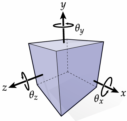
But sometimes we will encounter the Gimbal Lock!
Define rotation matrices for
For
Now, no matter how we adjust
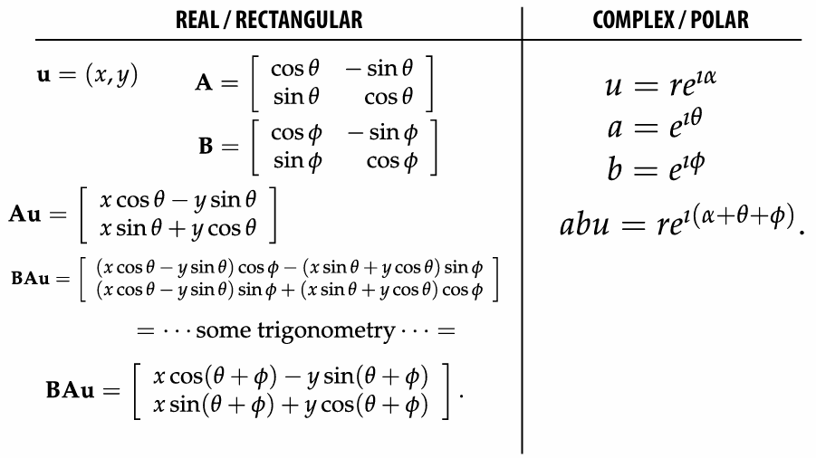
2.3.4 Complex Analysis
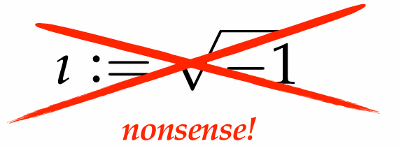
First, change the way of your thinking!
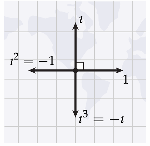
Instead, imagine it's just a quarter-turn in CCW direction:
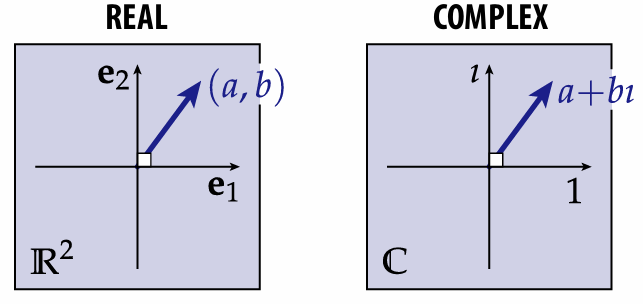
And complex numbers are just 2-vectors with
And the multiple operation is a little different, but the rest operations are the same:
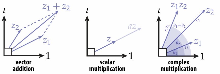
So:
*All the angle use rad.
2.3.5 Rotation: Matrices vs.Complex
2.3.6 Quaternions 四元数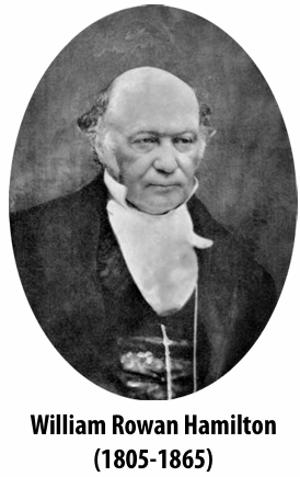
Hamilton’s insight: in order to do 3D rotations in a way that mimics complex numbers for 2D, actually need FOUR coordinates.
One real, and three imaginary:
*product no longer commutes!
To encode 3D points
where
A quaternion can be represented as a pair:
2.3.7 3D Rotations via Quaternions
Given axis
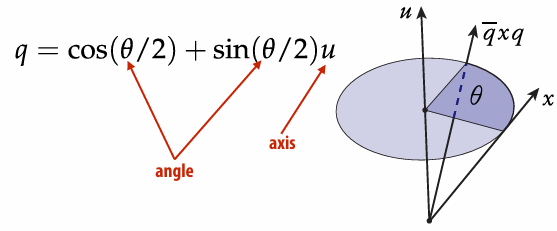
Here we consider the normal vector
2.4 Perspective Projection
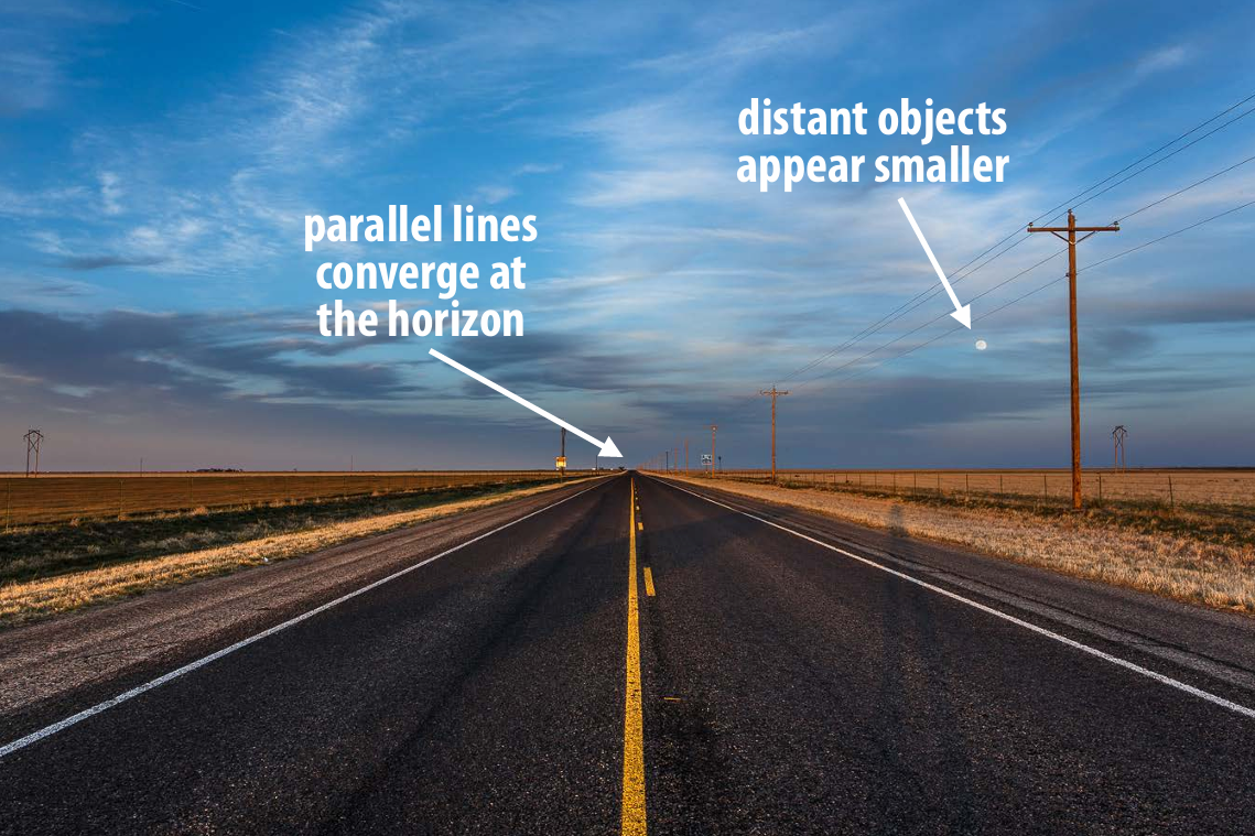
Distant objects appear smaller!
2.4.1 View Frustum
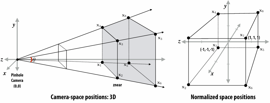
View frustum is region the camera can see:
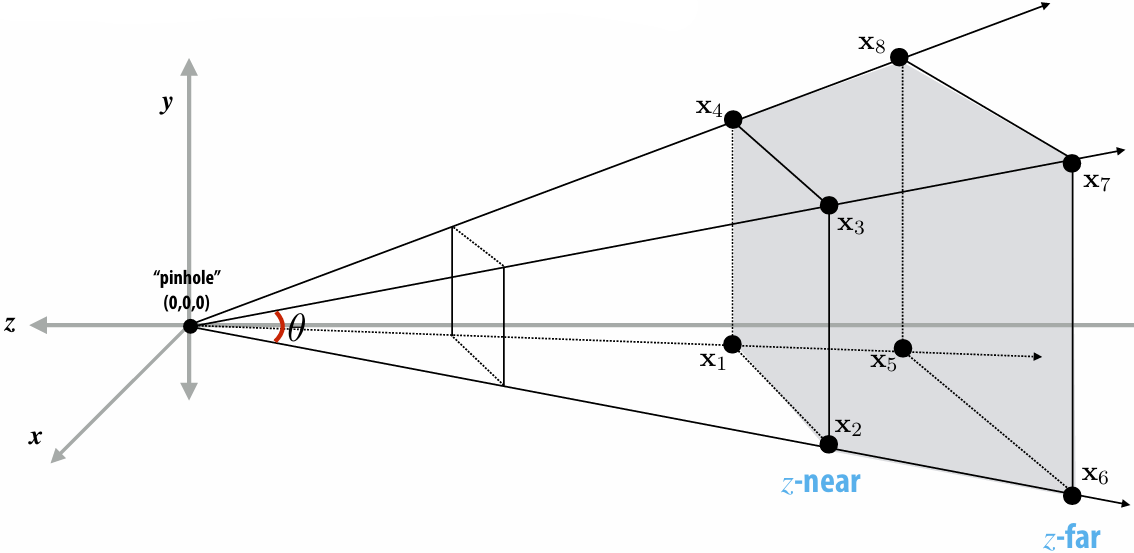
Top / bottom / left / right planes correspond to four sides of the image
Near / far planes correspond to closest/furthest thing we want to draw
2.4.2 Clipping
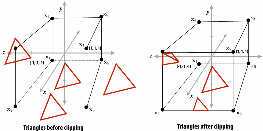
When objects are not visible to the camera / in view frustum, we clip it out!

*Also near/far clipping
2.4.3 Mapping Frustum to Unit Cube
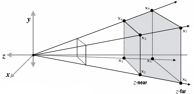
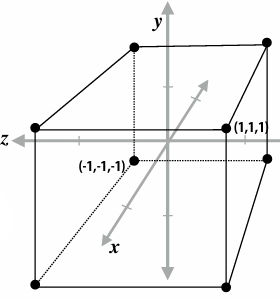
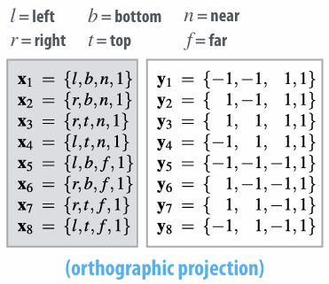
Solve
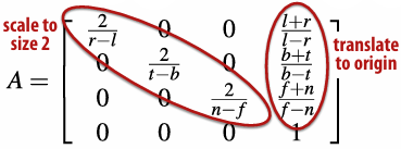
While we take perspective projection into account, it is:
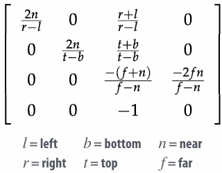
For derivation: OpenGL Projection Matrix
Warp Up:
2.5 Texture Mapping

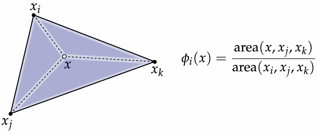
2.5.1 Barycentric Coordinates
Very useful for interpolation.
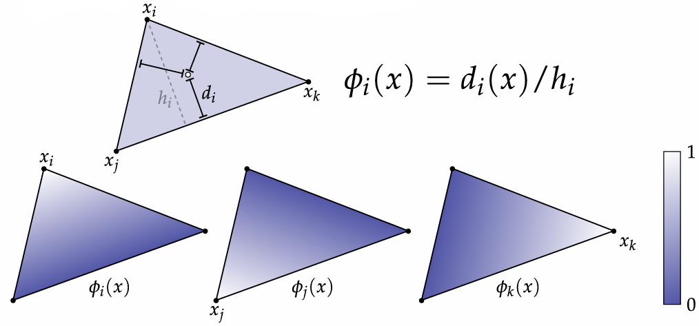
You can also regard it as the area proportions.
2.5.2 Perspective Correct Interpolation
Due to perspective projection (homogeneous divide), barycentric interpolation of values on a triangle with different depths is not an affine function of screen XY coordinates.
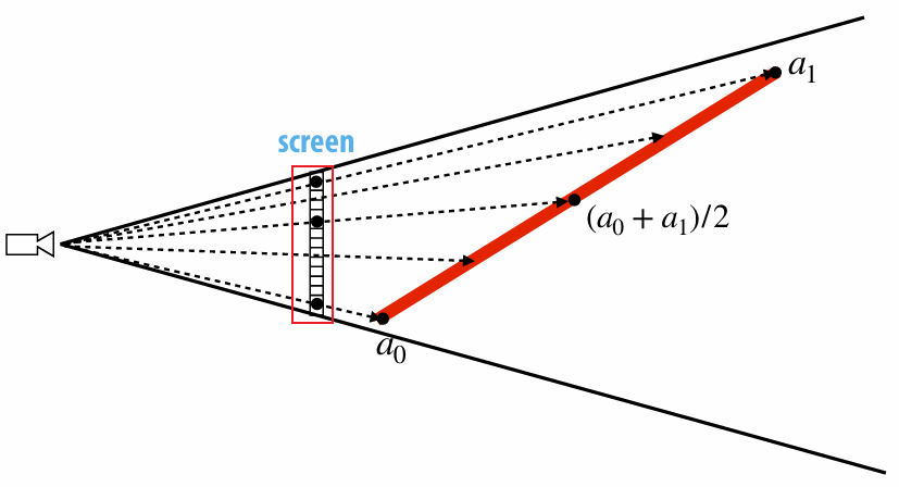
We want to interpolate attribute values linearly in 3D object space, not image space. If we compute barycentric coordinates using 2D (projected) coordinates, leads to (derivative) discontinuity in interpolation where quad was split:

How do we do?
Evaluate
Interpolate
Divide interpolated
For a derivation, see Microsoft Word - lowk_persp_interp_06.doc
2.5.3 Texture Coordinates
Texture coordinate define a mapping from surface coordinates to points in texture domain. Often defined by linearly interpolating texture coordinates at triangle vertices.
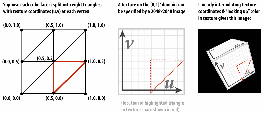
Each vertex has a coordinate
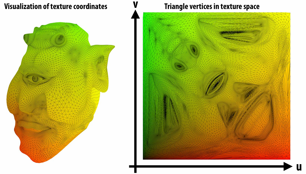 | 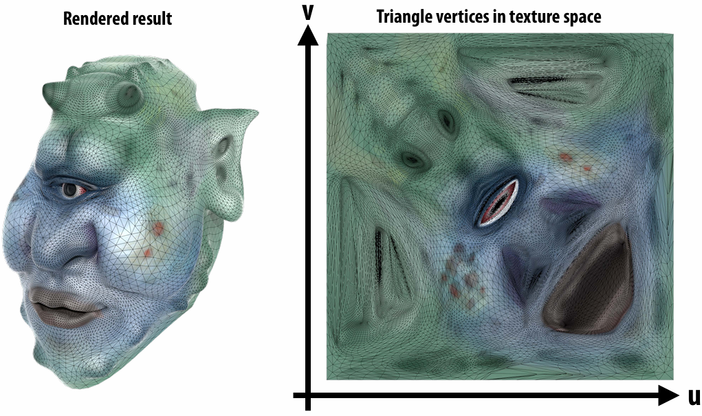 |
|---|
2.5.4 Magnification vs. Minification
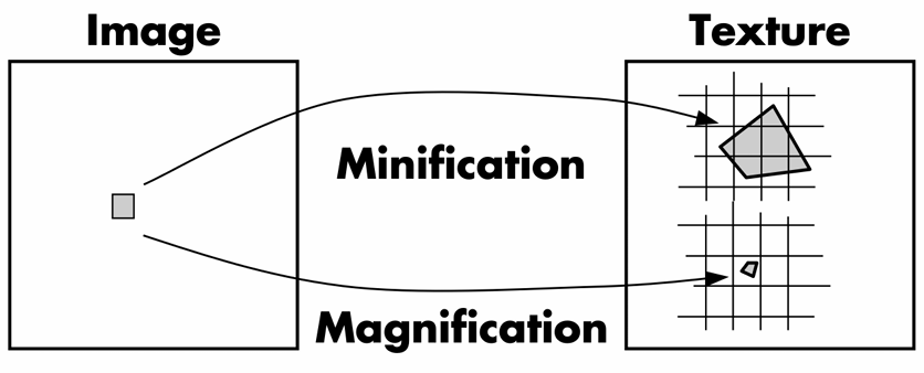
Magnification: camera is very close to scene object
Minification: scene objects are very far away
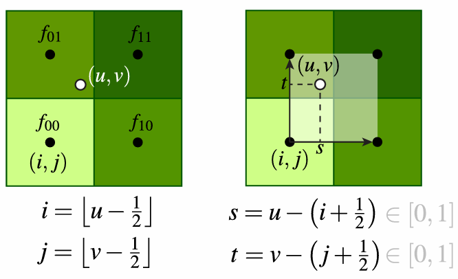
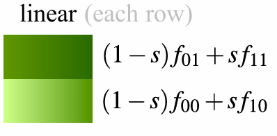
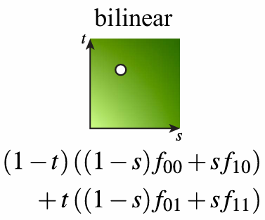
2.5.5 Bilinear Interpolation (Magnification)
2.5.6 MIP Map (Minification)
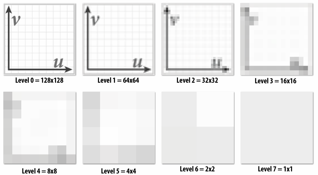
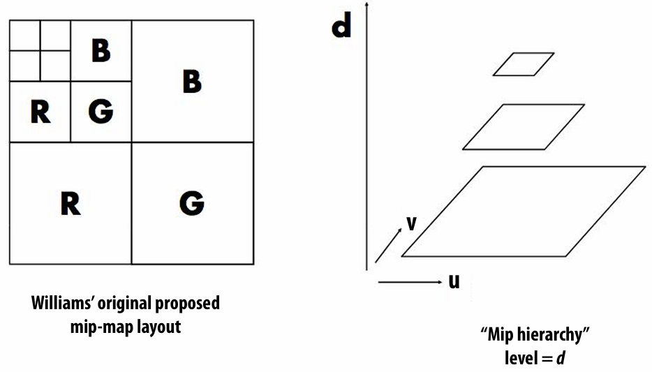
When a pixel on the screen covers many pixels of the texture, we can average texture values of these pixels, which is expensive to compute. So, we can precompute it and choose one demanded.
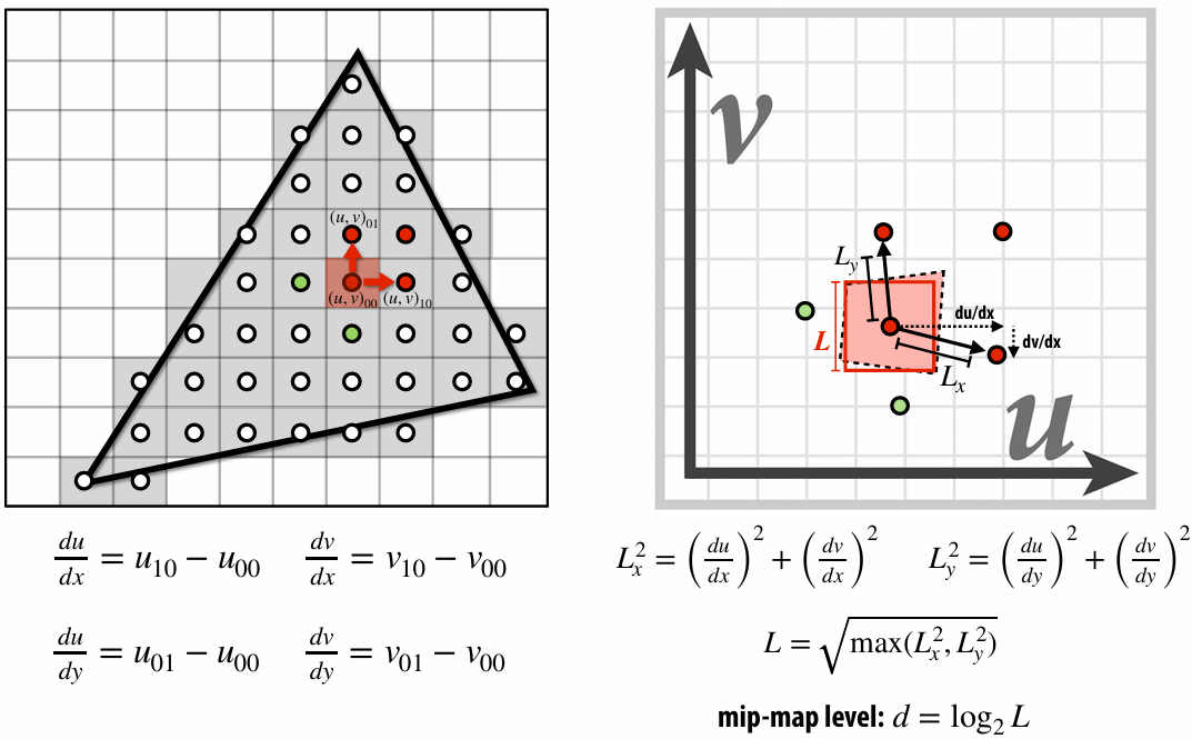
To get the mipmap level, we need to compute differences between texture coordinate values at neighboring samples.
2.5.7 Trilinear Interpolation for MIP Map
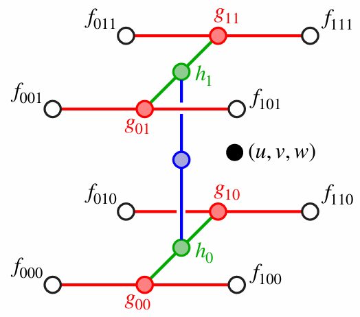
We can first bilinear interpolate with mipmap level, and then interpolate between two different levels.

2.5.8 Anisotropic Filtering
At grazing angles, samples may be stretched out by (very) different amounts along
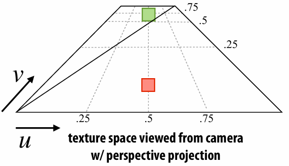
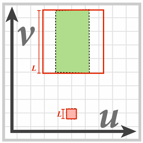
We can sample multiple times along the longer direction and less times along the short direction.
2.6 Depth and Transparency
2.6.1 Depth-Buffer
For each sample, depth-buffer stores the depth of the closest primitive seen so far.
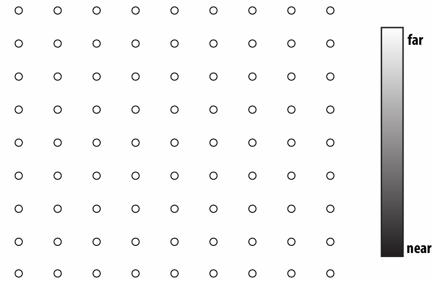
There are also color buffer, which can also be used for super-sampling, like (4 samples per pixel)
2.6.2 Compositing
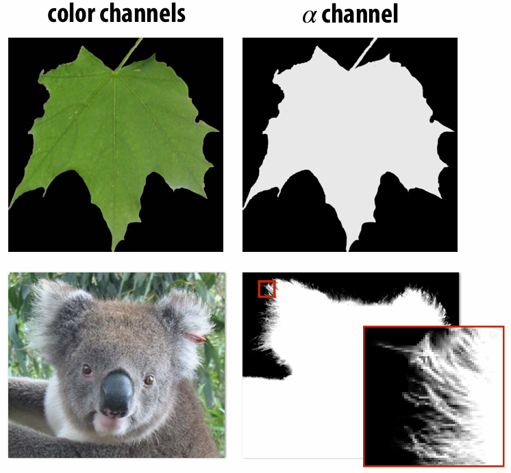
We can represent opacity as
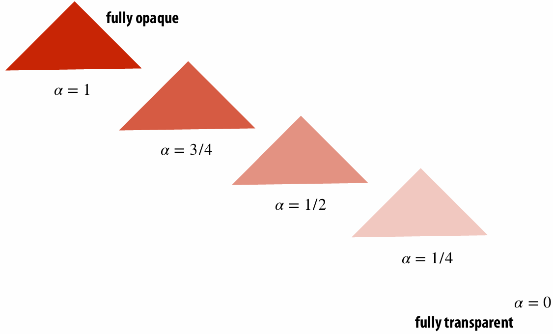
An image can have a
2.6.3 Fringing
| No fringing | Fringing |
|---|---|
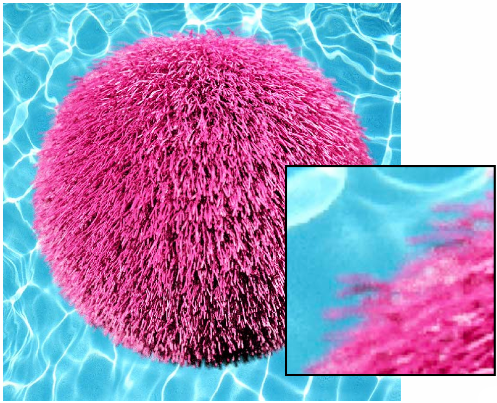 | 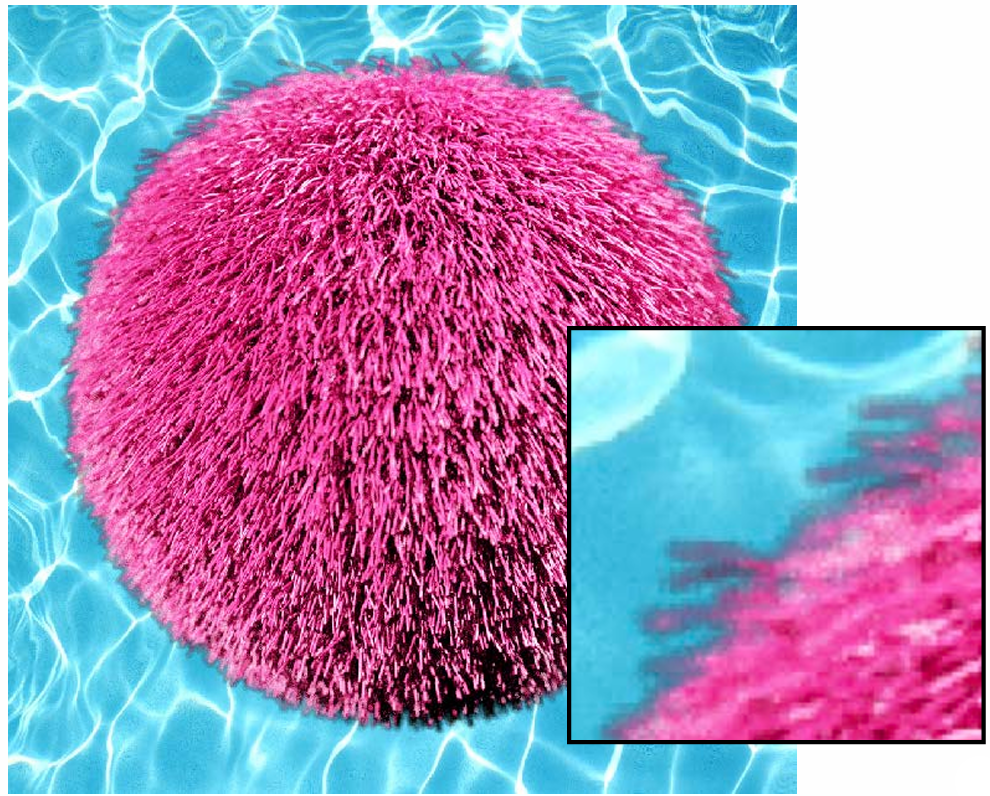 |
What cause this?
2.6.4 (Non-) Premultiplied Alpha
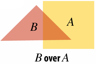
If we Composite image
| Non-premultiplied alpha | Premultiplied alpha |
|---|---|
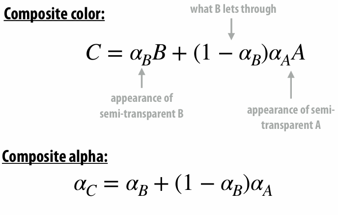 | 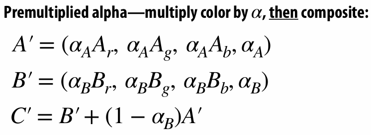   |
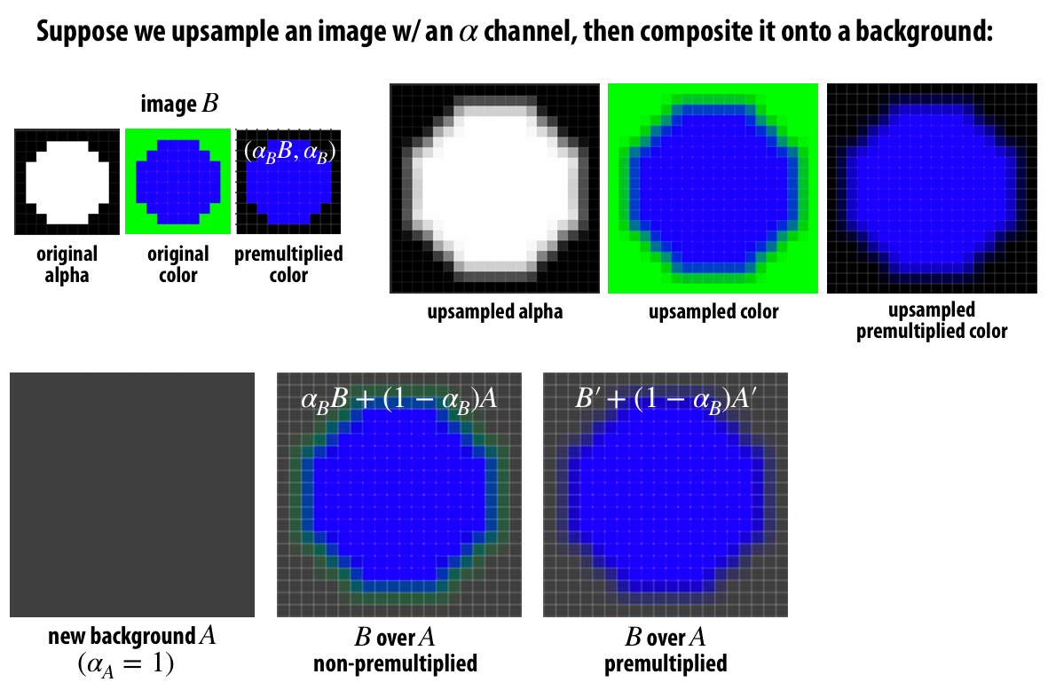
If we do not use the premulitplied alpha, there is fringe. Because the upsampled color mix the background color with original color. So we have to pre-multiplied color and then upsample it.
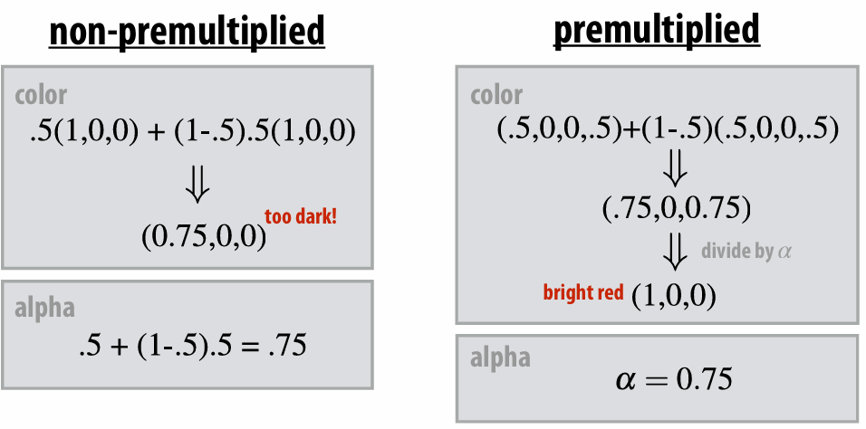
Premultiplied alpha is better!
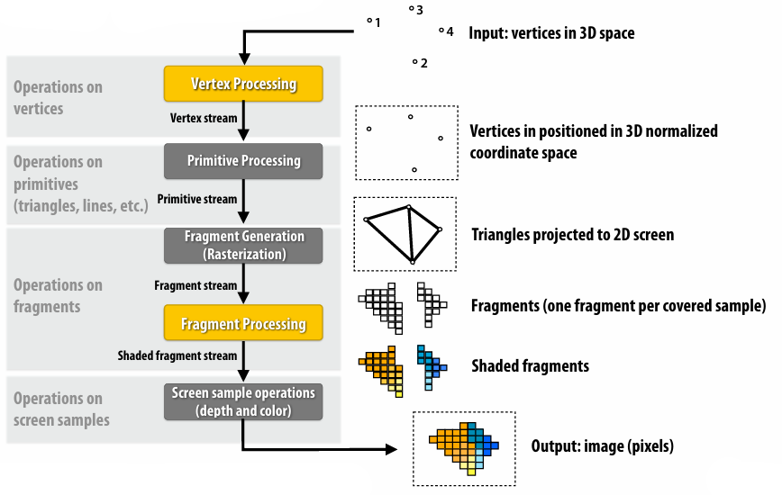
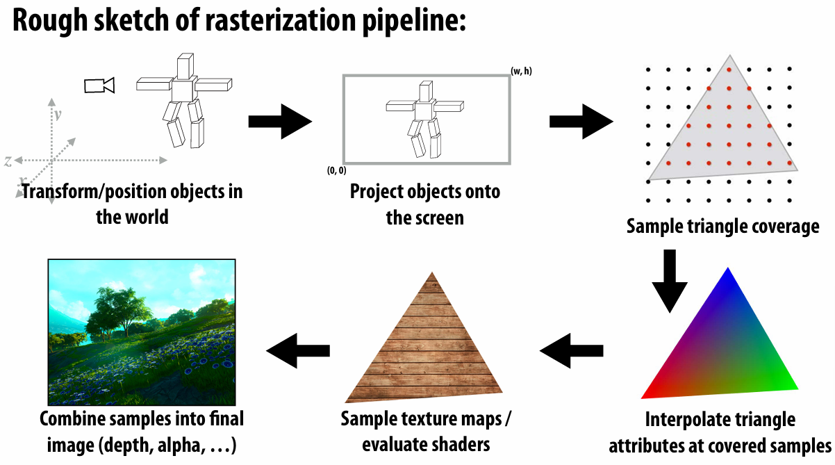
2.7 Rasterization Pipeline Summary
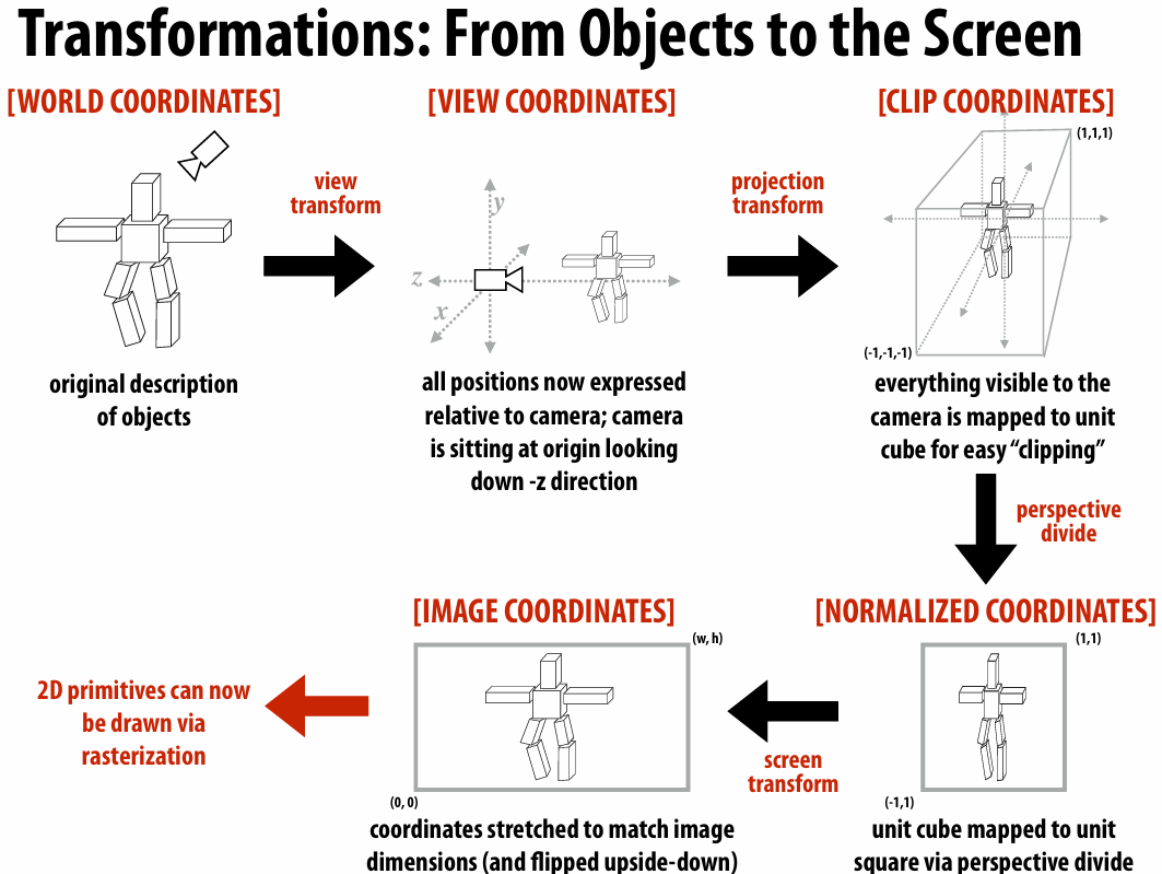
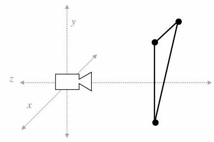
Transform triangle vertices into camera space
Apply perspective projection transform to transform triangle vertices into normalized coordinate space
Clipping
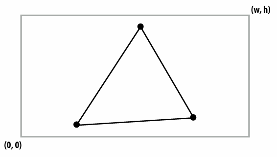
Transform to screen coordinates. Perform homogeneous divide, transform vertex xy positions from normalized coordinates into screen coordinates (based on screen w,h)
Setup triangle (triangle preprocessing). Before rasterizing triangle, can compute a bunch of data that will be used by all fragments
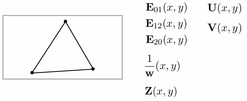
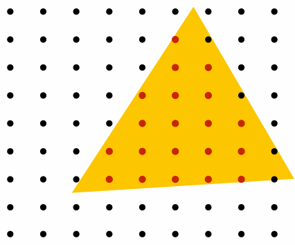
Sample coverage and compute triangle color at sample point
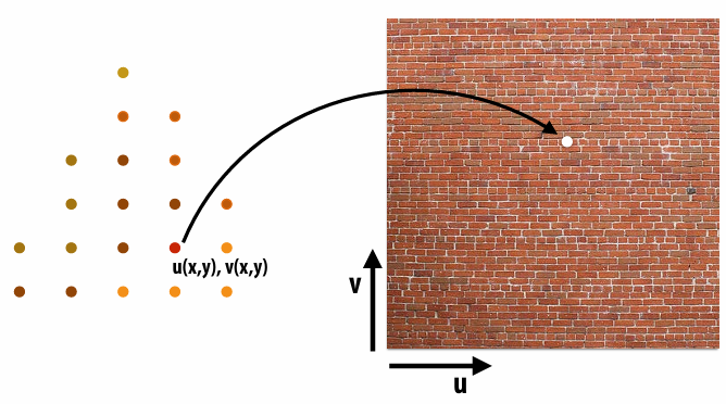
Perform depth test (if enabled)
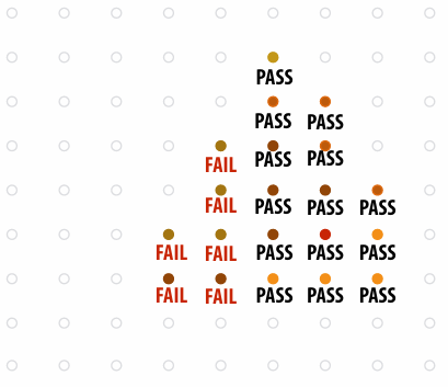
Update color buffer* (if depth test passed) (* Possibly using OVER operation for transparency)
OpenGL/Direct3D graphics pipeline:
3. Geometry
3.1 Encode Geometry
3.1.1 Implicit Representations
Points aren’t known directly, but satisfy some relationship. E.g., unit sphere is all points such that
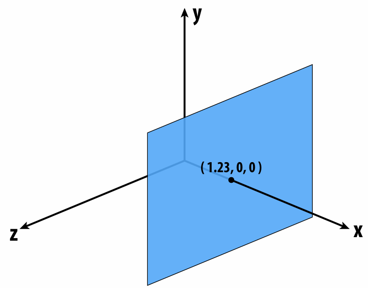
Now, find a point on the plane. And we can observe that implicit surfaces make sampling hard.
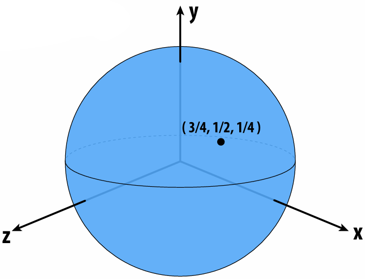
Now check if a point is inside or outside the unit sphere. And we can observe implicit surfaces make inside/outside tests task easy.
Common Implicit Representations:
Algebraic Surfaces
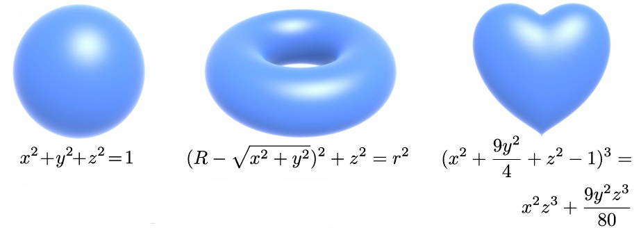
Constructive Solid Geometry (Boolean operations)

Blobby Surfaces (Gradually blend surfaces together)

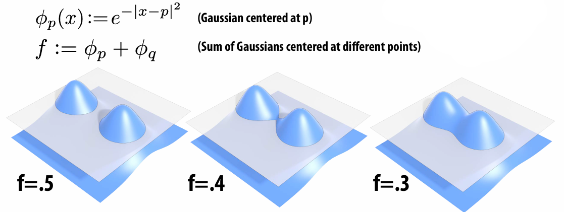
Blending Distance Functions

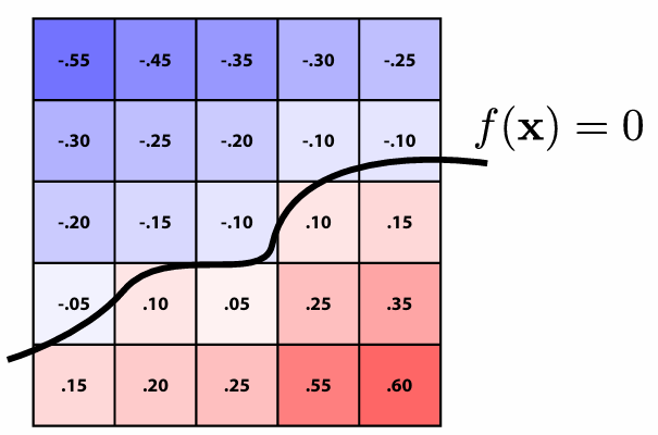
Level Set Methods (Surface is found where interpolated values equal zero )
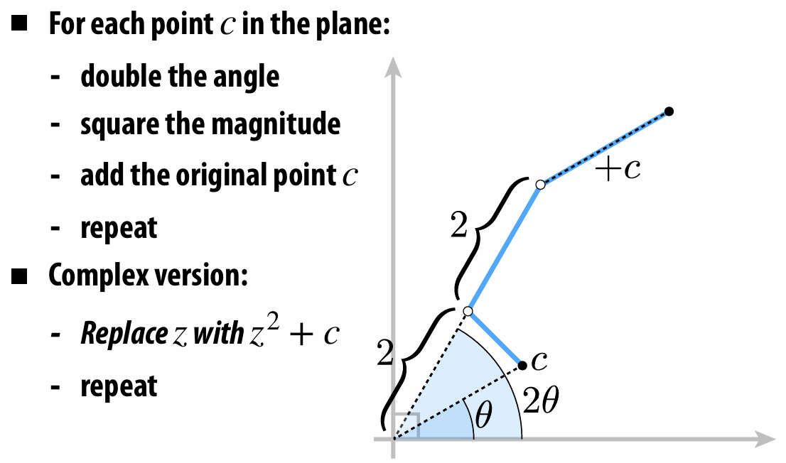
Mandelbrot Set
Pros:
description can be very compact (e.g., a polynomial)
easy to determine if a point is in our shape (just plug it in!)
other queries may also be easy (e.g., distance to surface)
for simple shapes, exact description/no sampling error
easy to handle changes in topology (e.g., fluid)
Cons:
expensive to find all points in the shape (e.g., for drawing)
very difficult to model complex shapes
3.1.2 Explicit Representations
All points are given directly. E.g., points on sphere are
Many explicit representations in graphics. Like triangle meshes, polygon meshes, subdivision surfaces, NURBS point clouds…
Unsimilar to implicit representations, explicit representations make sampling easy but inside/outside test hard.
Common Explicit Representations:
Point Cloud
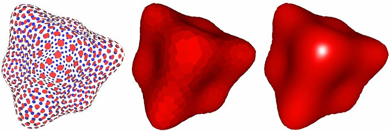
Polygon Mesh ( Store vertices and polygons)
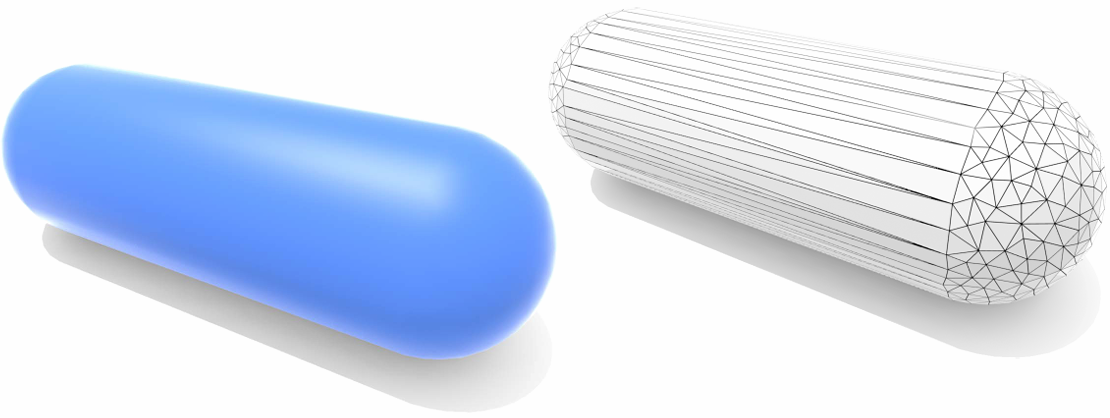
Bézier Curves/Surfaces
Bernstein Basis:
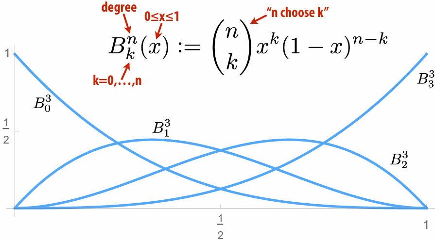
It can use to interpolate different points:

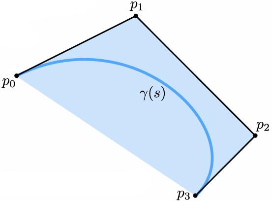
We can piece together many Bézier curves to interpolate lots of points (because High-degree Bernstein polynomials don’t interpolate well):

Bézier Patches is Bézier patch is sum of (tensor) products of Bernstein bases:
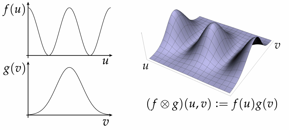
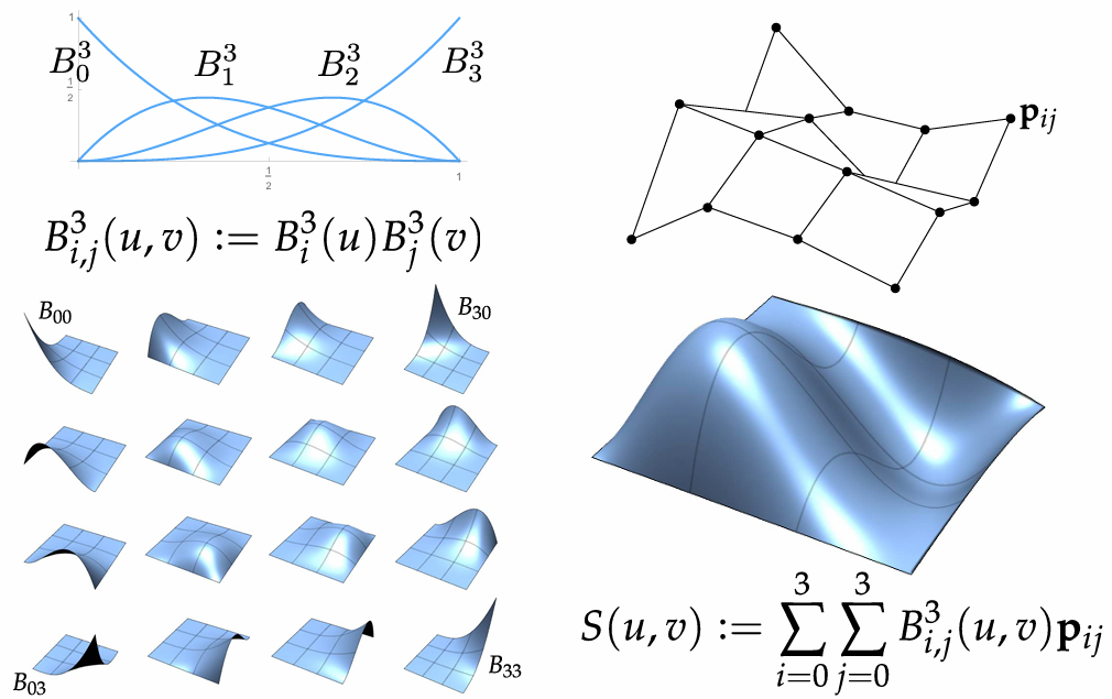
By connecting Bézier curves, can connect Bézier patches to get a surface:
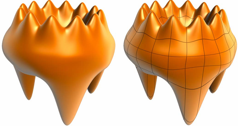
Basically, it is weight-average points (2D, 3D)
Rational B-Splines
Bézier can’t exactly represent conics—not even the circle!
Solution: interpolate in homogeneous coordinates, then project back to the plane:
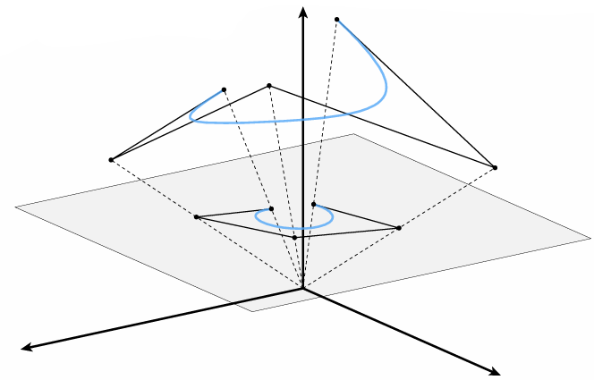
NURBS: (N)on-(U)niform (R)ational (B)-(S)pline
knots at arbitrary locations (non-uniform)
expressed in homogeneous coordinates (rational)
piecewise polynomial curve (B-Spline)
w is homogeneous coordinate, controlling "strength" of a vertex
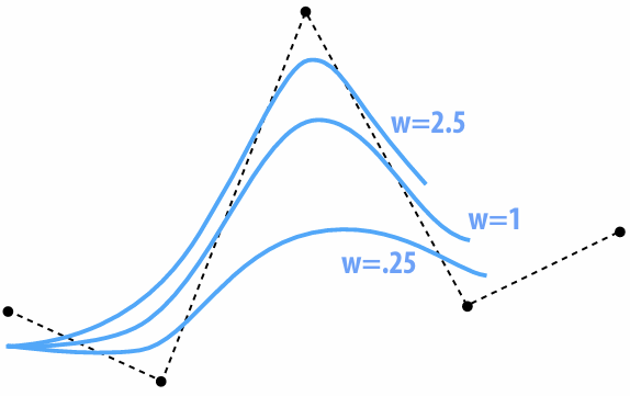
We can use tensor product to the NURBS curve


Subdivision:
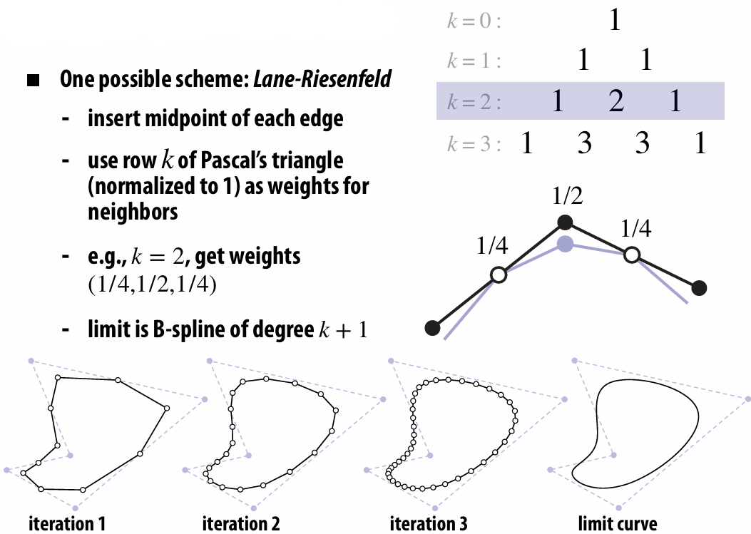
3.1.3 Summary
Some representations work better than others—depends on the task!
3.2 Meshes and Manifolds
3.2.1 Manifold Assumption
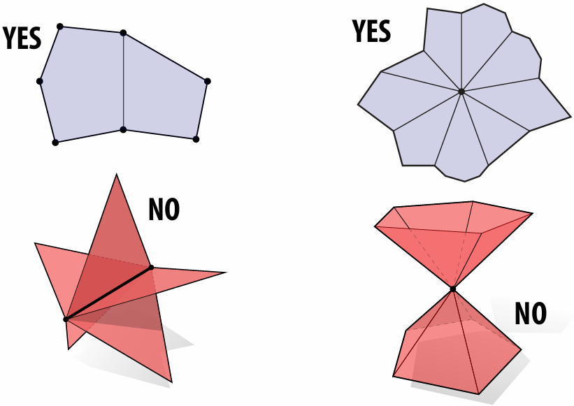
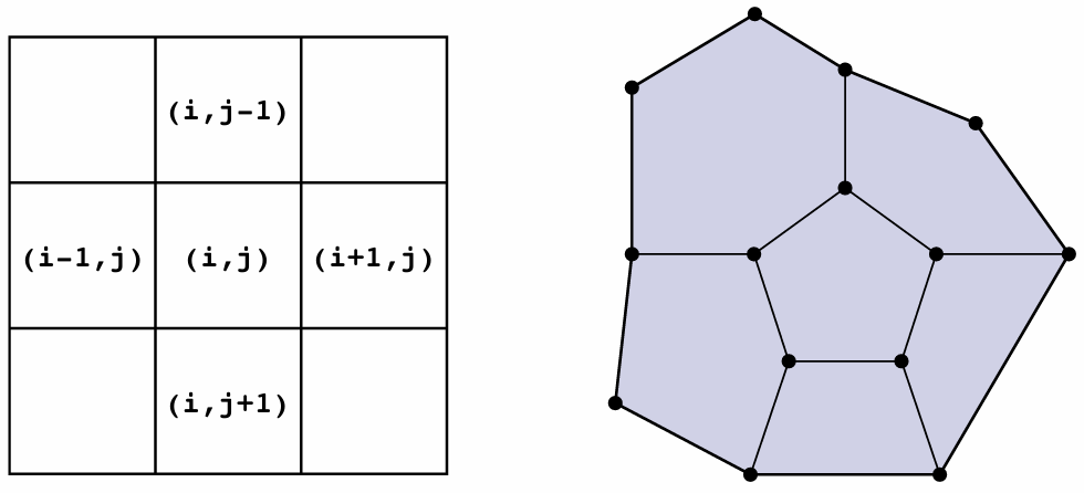
If you zoom in far enough, can draw a regular coordinate grid. (Very rough definition)
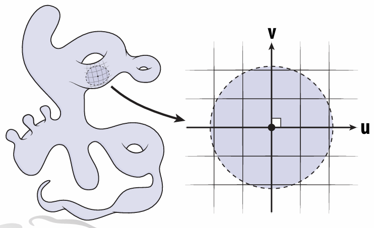
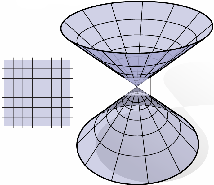
This is not manifold:
Which of shapes are manifold?
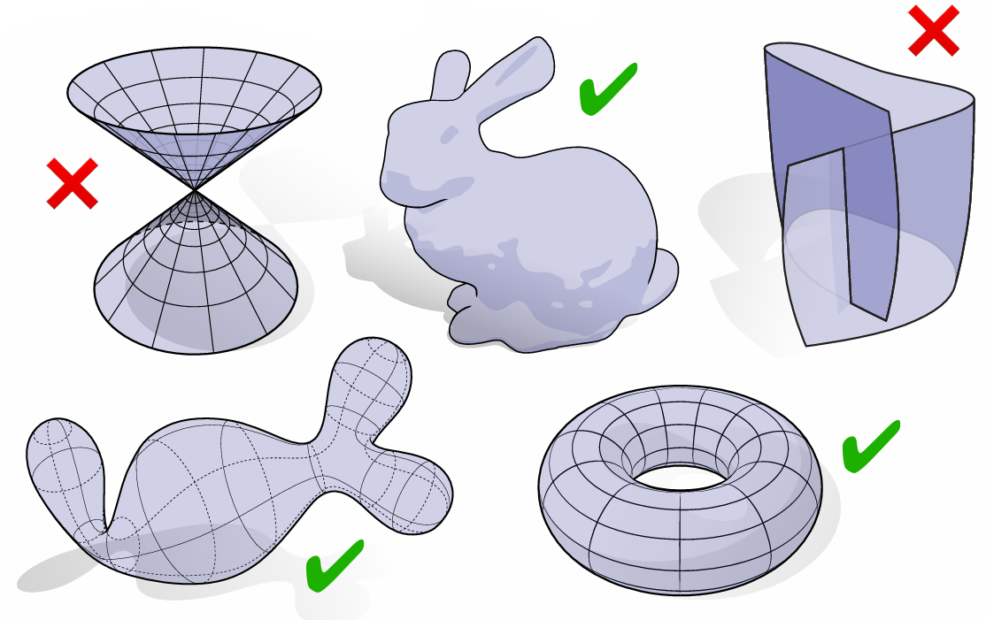
Or, we can say: A manifold polygon mesh has fans, not fins
Every edge is contained in only two polygons (no “fins”)
The polygons containing each vertex make a single “fan”
3.2.2 Why Do We Need Manifold?
To make some assumptions about our geometry to keep data structures/algorithms simple and efficient
In many common cases, doesn’t fundamentally limit what we can do with geometry
3.2.3 Halfedge Data Structure
*There are lots data structure can be used to store meshes, here we only talk about halfedge.
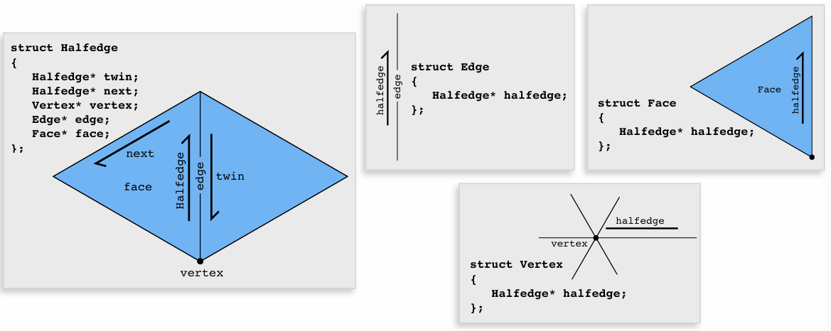
Halfedge makes mesh traversal easy:
Visit all vertices of a face
1Halfedge* h = f->halfedge;2do {3h = h->next;4h->vertex...5} while (h != f-> halfedge);Visit all neighbors of a vertex:
xxxxxxxxxx41Halfedge* h = v->halfedge;2do {3h = h->twin->next;4} while (h != v-> halfedge);…
Halfedge connectivity is always manifold:
Keep following
next, and you’ll get faces.Keep following
twinand you’ll get edges.Keep following
next->twinand you’ll get vertices.
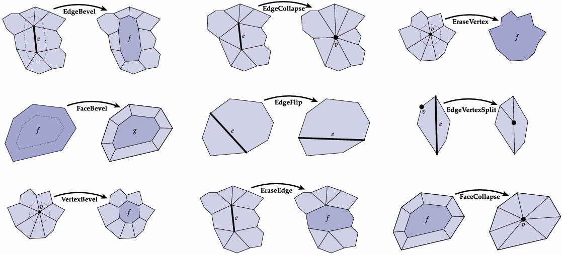
3.2.4 Halfedge Meshes Edition
Edge Flip

Edge Split

Edge Collapse

More…
3.3 Digital Geometry Processing
3.3.1 Remeshing as Resampling
Undersampling destroys features
Oversampling bad for performance
We need "good sampling"—"good" mesh. We need good approximation of original shape! Keep only elements that contribute information about shape. Add additional information where, e.g., curvature is large.
Vertices exactly on the surface doesn't mean it is a good approximation.
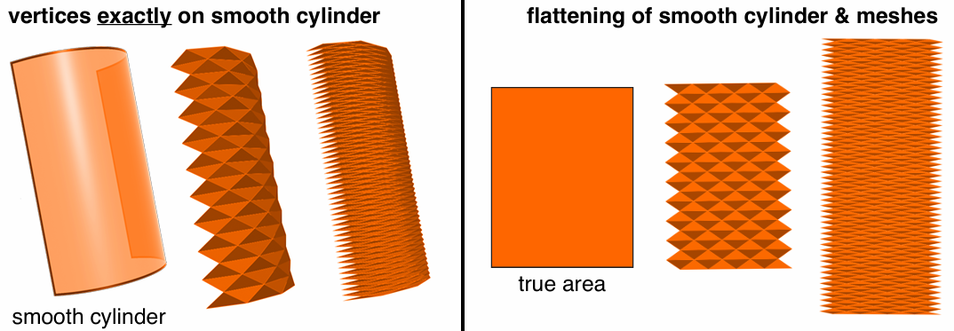
(Some attributes, like normal is not good).
One rule of thumb: triangle shape—Delaunay
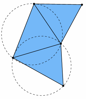
For any triangle in the decomposition, the interior of its circumcircle does not contain any other point.
Another rule of thumb: regular vertex degree: Degree 6 for triangle mesh, 4 for quad mesh

3.3.2 Upsampling via (Catmull-Clark/Loop) Subdivision
There are lots of ways to do the subdivision.
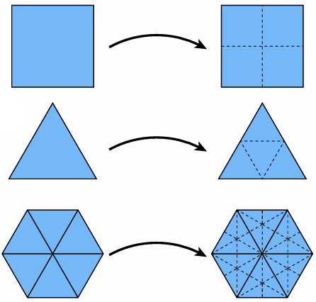
Catmull-Clark subdivision
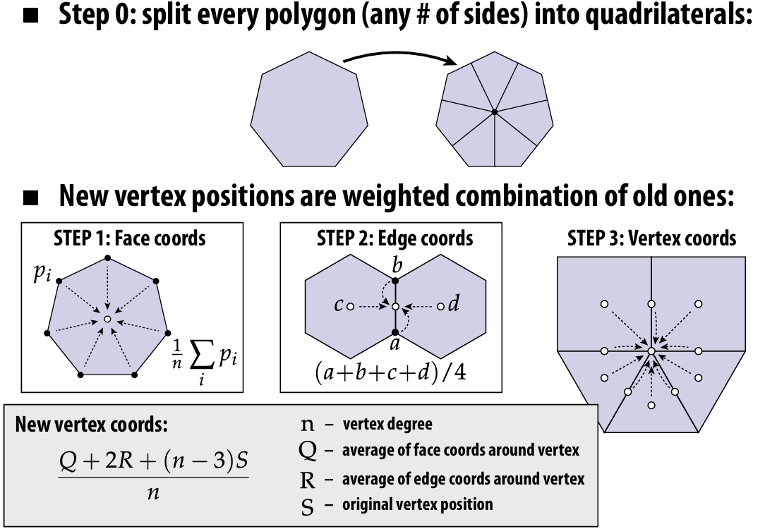
For more detailed tutorial: Catmull-Clark Subdivision: The Basics – CodeItNow
Loop Subdivision

We can use edge operations to complete the subdivision:
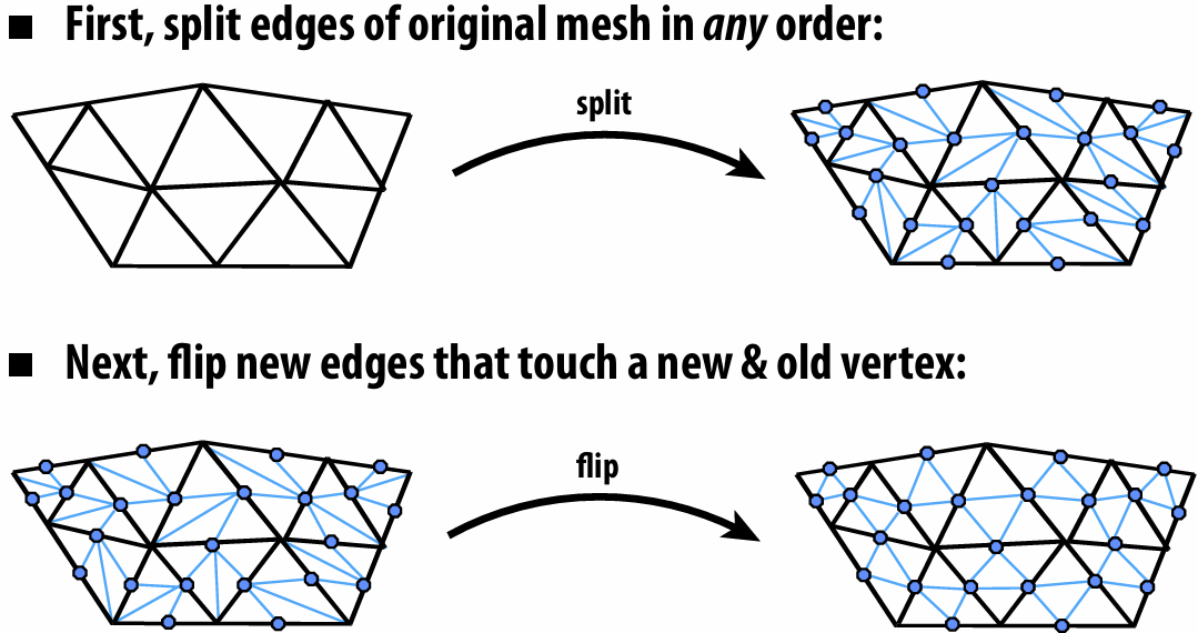
(Don’t forget to update vertex positions!)
3.3.3 Simplification via Edge Collapse
Basically, we assign each edge a cost, collapse the edge with least cost, and repeat until we reach the target.

And we use Quadric Error Metrics to determine edge's cost.
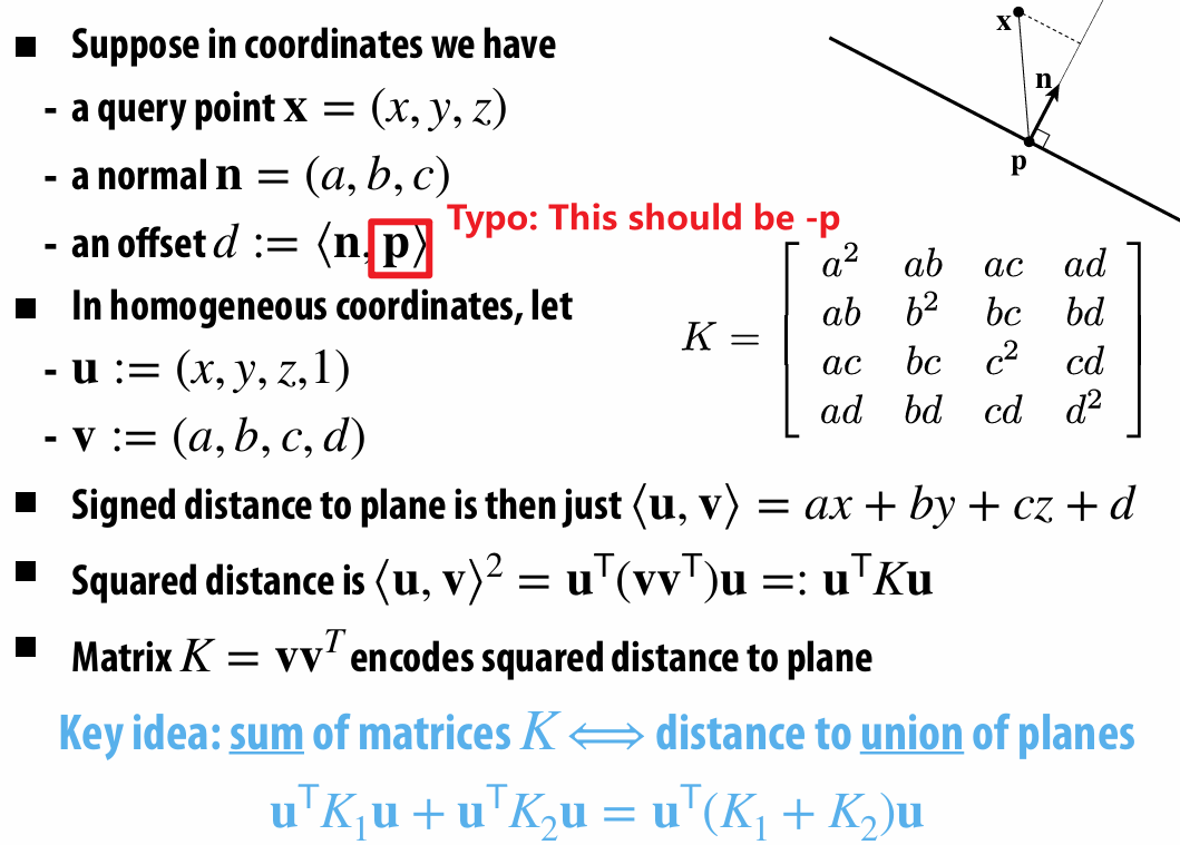
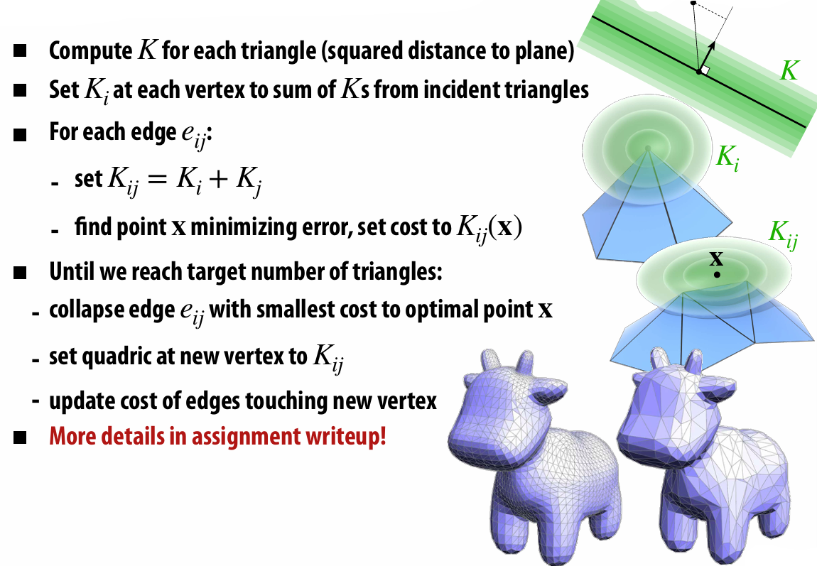
For a derivation, see Scotty3D_Benky/assignments/A2/simplify.md at main · tbbbk/Scotty3D_Benky
3.3.4 Isotropic Remeshing Algorithm
How to make triangles uniform shape & size?
Repeat four steps:
Split any edge over 4/3rds mean edge length
Collapse any edge less than 4/5ths mean edge length
Flip edges to improve vertex degree
Center vertices tangentially
3.5 Geometric Queries
3.5.1 Ray Equation
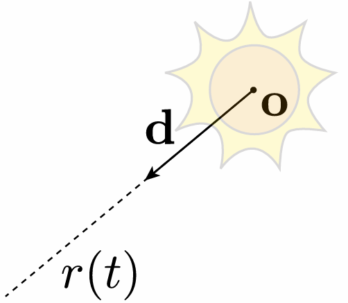
3.5.2 Intersection
For implicit surface intersection,
For explicit surface intersection (e.g. triangle), things become much harder and we do care about performance!
We will introduce Spatial Acceleration Data Structures!
3.6 Spatial Acceleration Data Structures
What we care about most is the ray-triangle intersection!
3.6.1 Affine Map for Triangle
We can parameterize triangle given by vertices
Now it's like:

So now the ray-triangle intersection is like:
We only need to solve for
3.6.2 Bounding Box
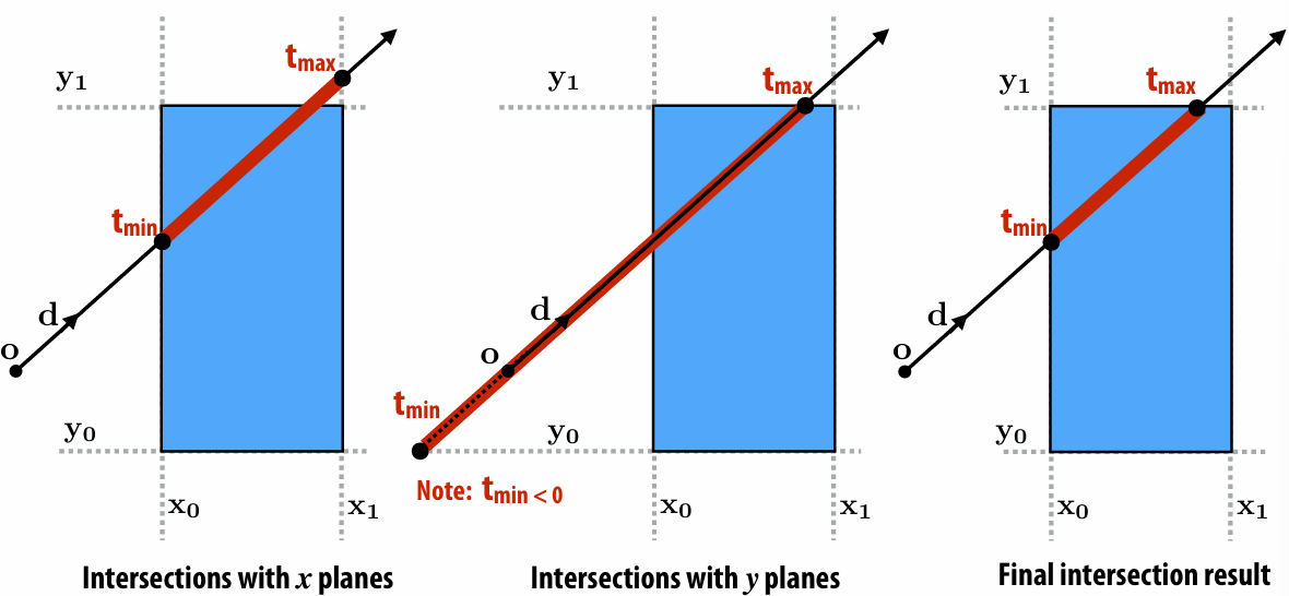
We can pre-compute a bounding box around all primitives. If a ray intersect with a bounding box, then we test each primitives within this bounding box to avoid meaningless tradeoff.
Then use calculate the ray-axis-aligned box intersection:
The uniform equation is:
Solve for the
More examples:
3.6.3 Bounding Volume Hierarchy (BVH)
BVH implementation assignment is really the pain in the ass…
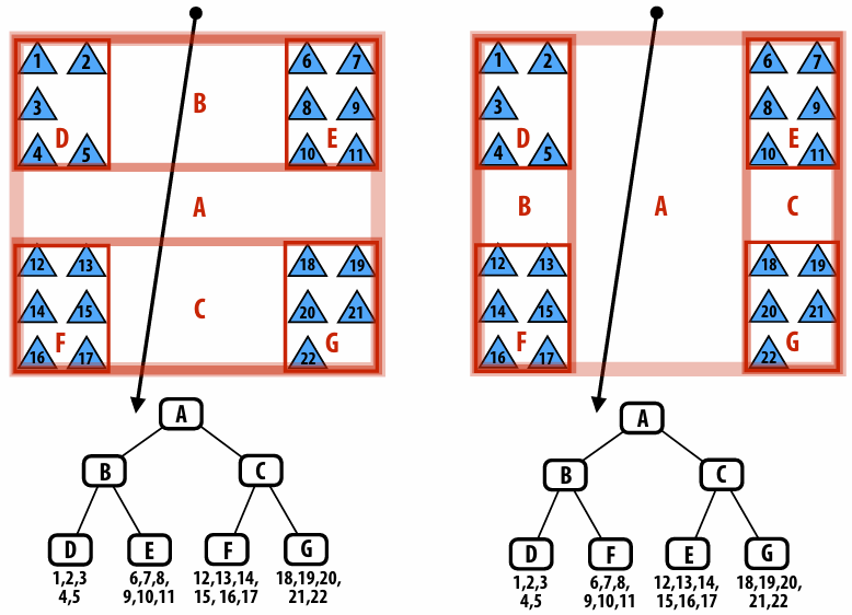
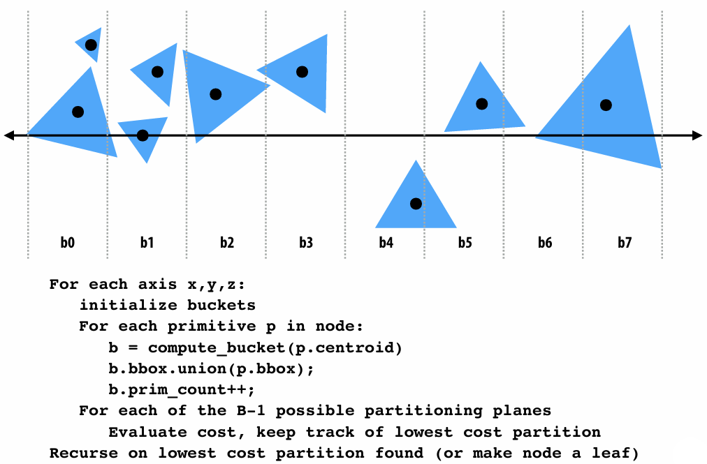
How do we build the better BVH? We need a better partition.
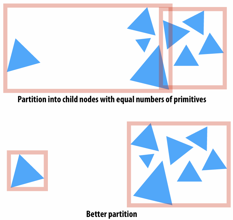
A good partitioning minimizes the cost of finding the closest intersection of a ray with primitives in the node.
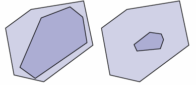
The pipeline about building BVH:
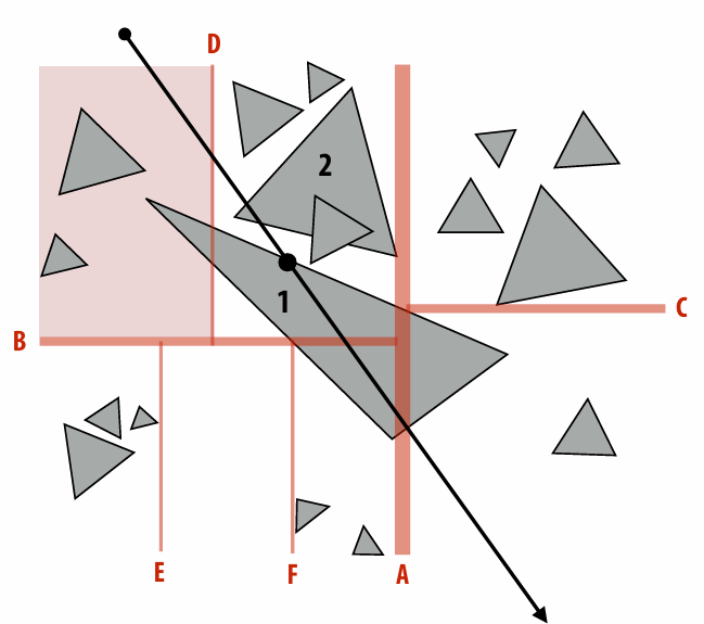
Beside BVH, there are also lots data structure to accelerate:
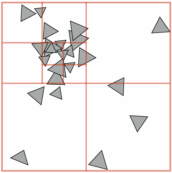
K-D tree
Uniform grid
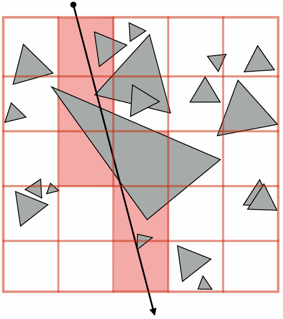
Heuristic: Choose number of voxels ~ total number of primitives
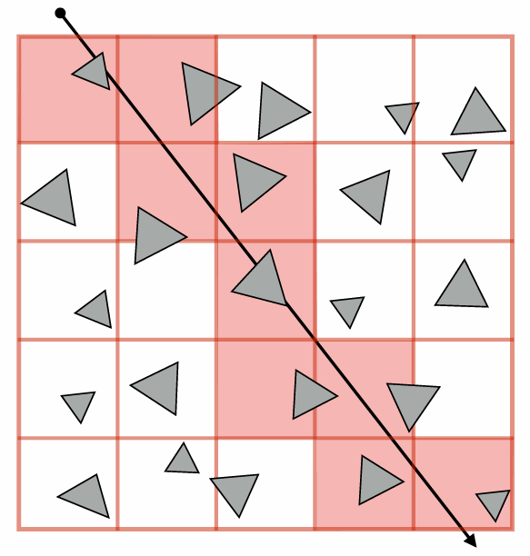
Quad-tree / octree
4. Ray Tracing
4.1 Color
For the color section, I literally omit a lot of contents… Because I didn't listen to the color lecture very carefully orz
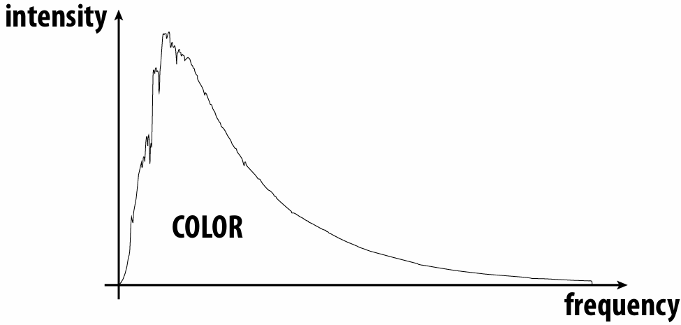
Light is oscillating electric & magnetic field.
KEY IDEA: frequency determines color of light
4.1.1 Intensity or Absorption
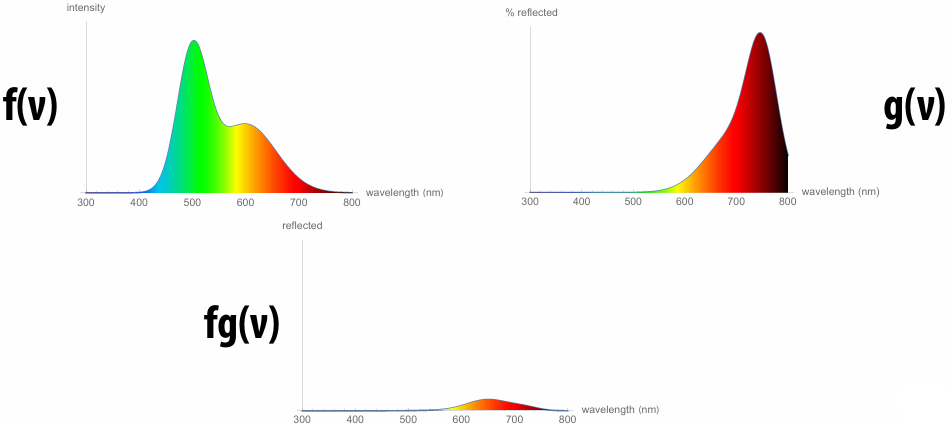
4.1.2 Emission and Reflection
4.1.3 Color Models
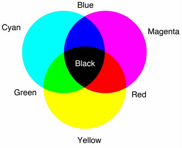
RGB
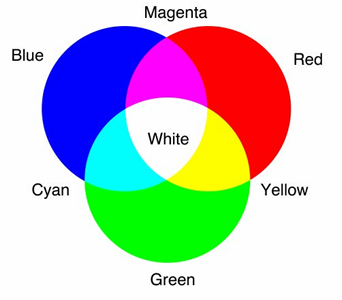
CMYK
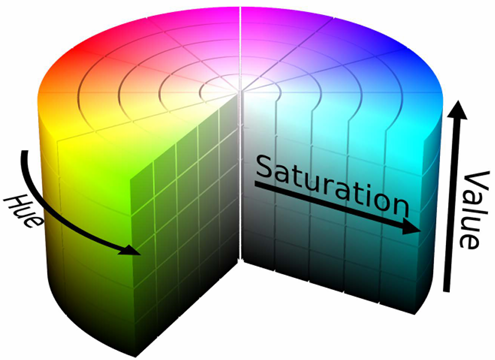
HSV
SML
XYZ
…
4.1.4 Y’CbCr
Y’ = luma: perceived luminance (same as L* in CIELAB)
Cb = blue-yellow deviation from gray
Cr = red-cyan deviation from gray
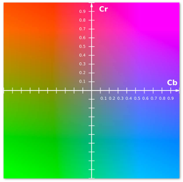
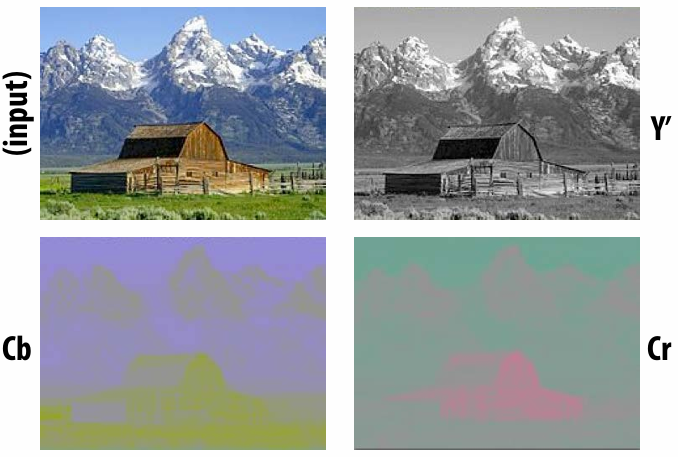
4.2 Radiometry
4.2.1 Photon
Imagine every photon is a little rubber ball hitting the scene.
4.2.2 Radiant Energy
This it "the number of hits". Energy for single photon:
where:
4.2.3 Radiant Flux
Energy per unit time (Watts) received by the sensor (or emitted by the light)
4.2.4 Irradiance
Area density of radiant flux, given a senor of with area
Irradiance (
4.2.5 Lambert's Law
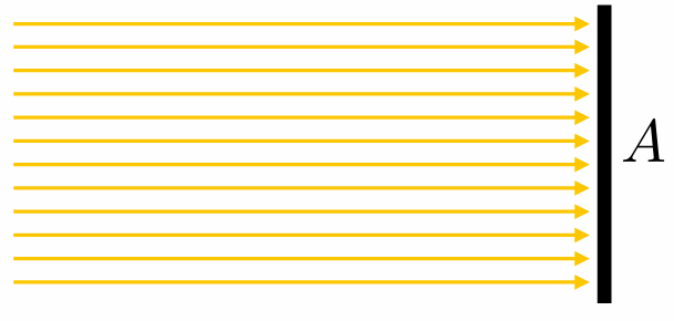 | 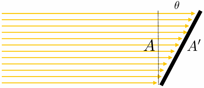 |
|---|---|
4.2.6 Irradiance Falloff with Distance
Given flux
Since same amount of energy is distributed over larger and larger spheres, has to get darker quadratically with distance.
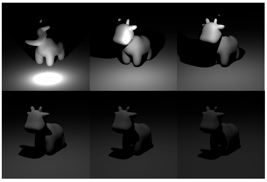
4.2.7 Solid Angles
| Radians | Steradians |
|---|---|
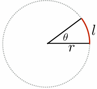 | 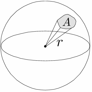 |
Differential solid angle:
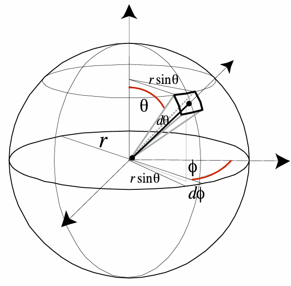
4.2.8 Radiance
Radiance is the solid angle density of irradiance:
where

In other words, radiance is energy along a ray defined by origin point p and direction
Energy per unit time per unit area per unit solid angle…!
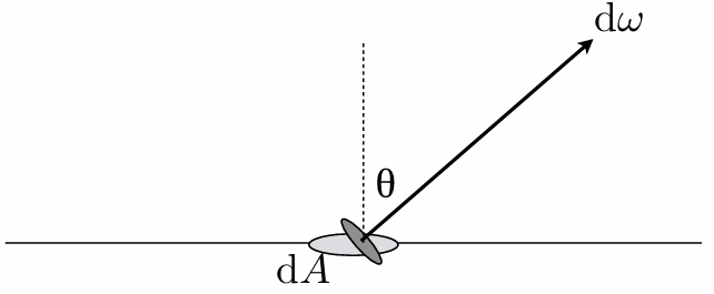
Surface radiance:
Reminder: Often need to distinguish between incident radiance and exitant radiance functions at a point on a surface. In general:
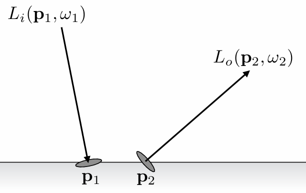
4.2.9 Spectral Radiance

Now, the radiance is radiant energy per unit time per unit area per unit solid angle. If we wanna get the COLOR, we need to add a "per unit wavelength"
4.2.10 Ambient Occlusion
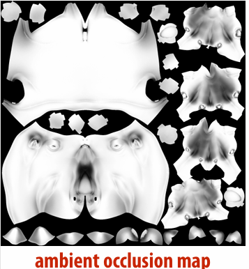
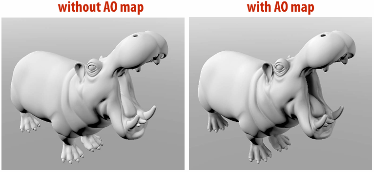
Assume spherical (vs. hemispherical) light source, “at infinity”. Irradiance is now rotation, translation invariant. Can pre-compute, “bake” into texture to enhance shading
4.2.11 Radiant Intensity
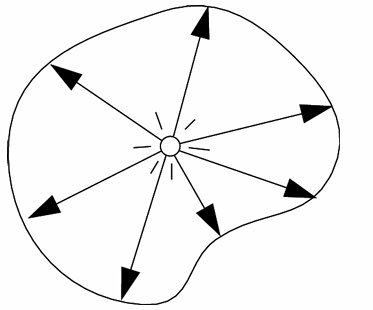
Power per solid angle emanating from a point source.
4.3 The Rendering Equation

4.3.1 Recursive Raytracing
Basic strategy: recursively evaluate rendering equation!
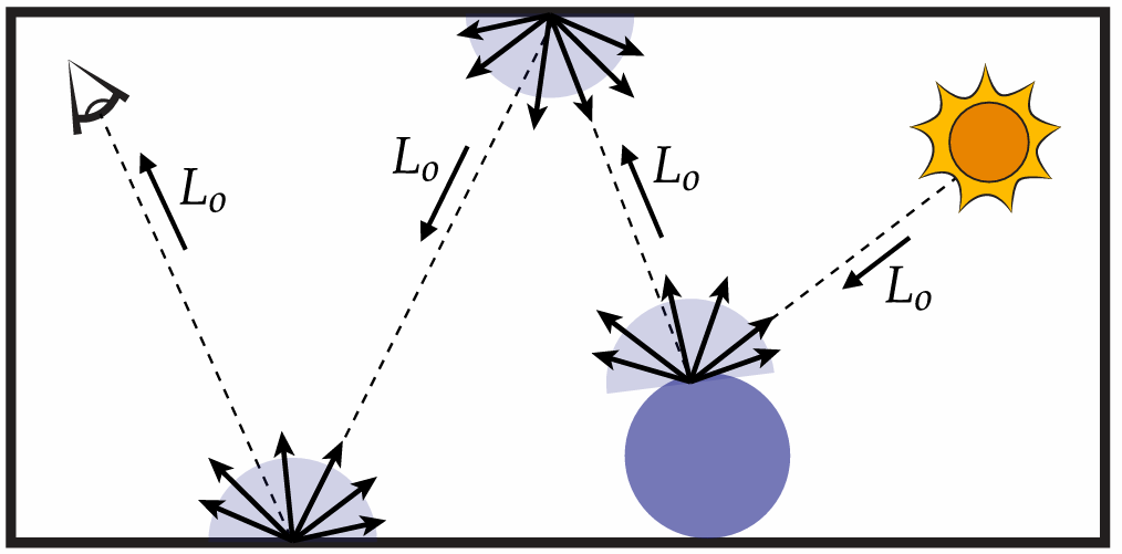
Renderer measures radiance along a ray:
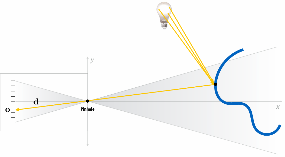
4.3.2 Reflection
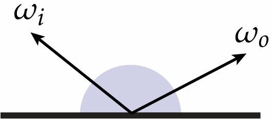
When the ray bounce in scene, how does the reflection of light affect the outgoing radiance?

What we are talking about is the scatter function in the rendering equation. Choice of reflection function determines surface appearance.
Some basic reflection functions:
| Reflection | Examples |
|---|---|
| Ideal specular: Perfect mirror | 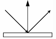 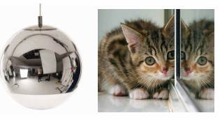 |
| Ideal diffuse: Uniform reflection in all directions | 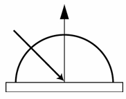  |
| Glossy specular: Majority of light distributed in reflection direction | 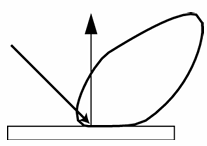 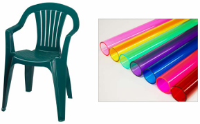 |
| Retro-reflective: Reflects light back toward source | 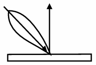 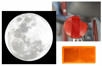 |
4.3.3 Models of Scattering
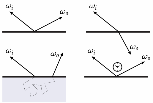
What goes in must come out! (Total energy must be conserved)
4.3.4 BRDF (Bidirectional Reflectance Distribution Function)
It encodes behavior of light that “bounces off” surface and calculate, when given incoming direction
Radiometric description of BRDF:For a given change in the incident irradiance, how much does the exitant radiance change?
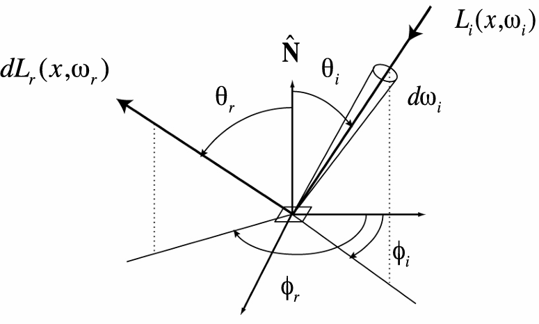
Common BRDF:
Lambertian reflection
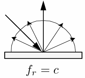
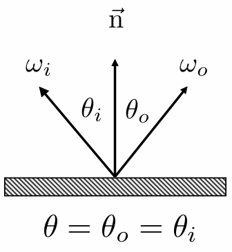
Specular reflection
Refraction:
Snell's Law
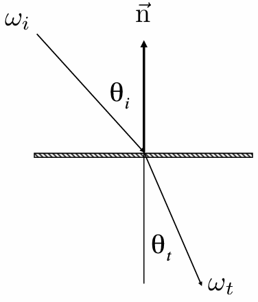
Law of refraction: solve the
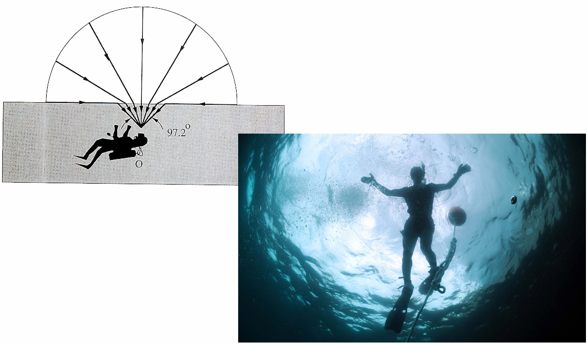
Optical manhole: Only small “cone” visible, due to total internal reflection (TIR) (When light is moving from a more optically dense medium to a less optically dense medium, light incident on boundary from large enough angle will not exit medium.)
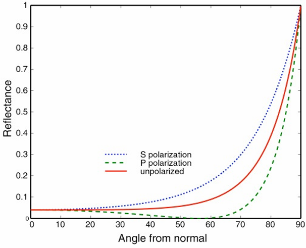
Fresnel reflection: Many real materials: reflectance increases w/ viewing angle

Anisotropic reflection: Reflection depends on azimuthal angle
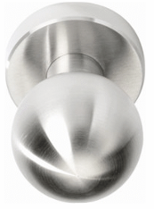
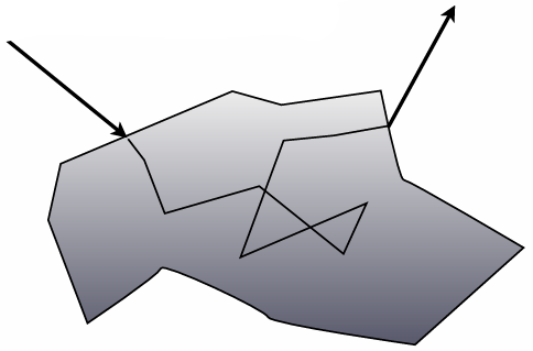
4.3.5 Subsurface scattering
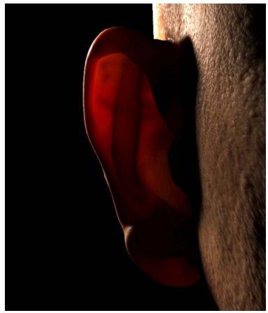
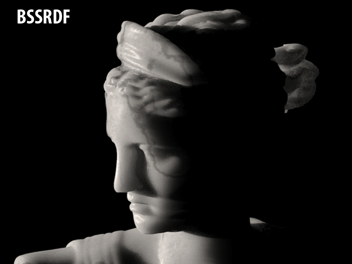
BSSRDF:
 |  |
|---|
5. Optimization for Ray Tracing
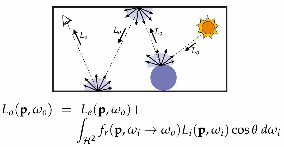
5.1 Numerical Integration
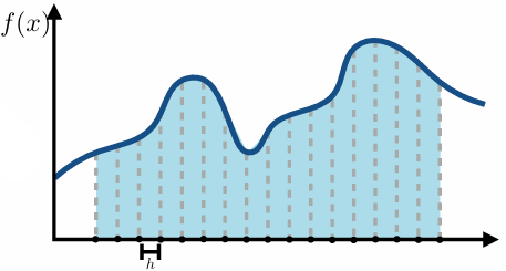
Basic idea:
integral is “area under curve”
sample the function at many points
integral is approximated as weighted sum
5.1.1 Gauss Quadrature
For any polynomial of degree n, we can always obtain the exact integral by sampling at a special set of n points and taking a special weighted combination.
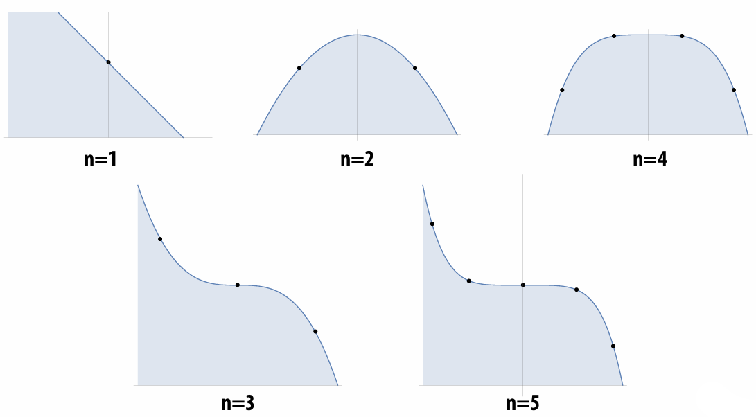
Weighted combination of sample points.
Key idea so far: To approximate an integral, we need
quadrature points
weights for each point
5.1.2 Trapezoid rule
Approximate integral of
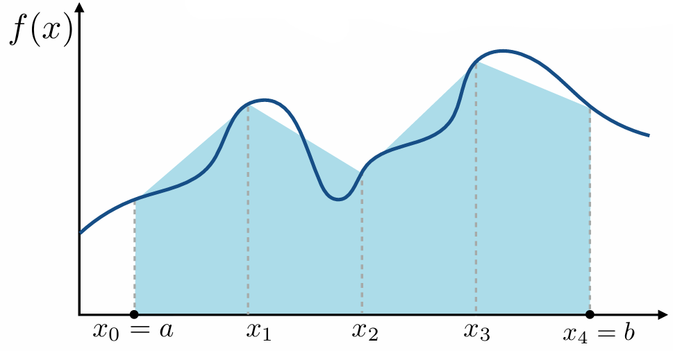
Work:
Error:
How about 2D?
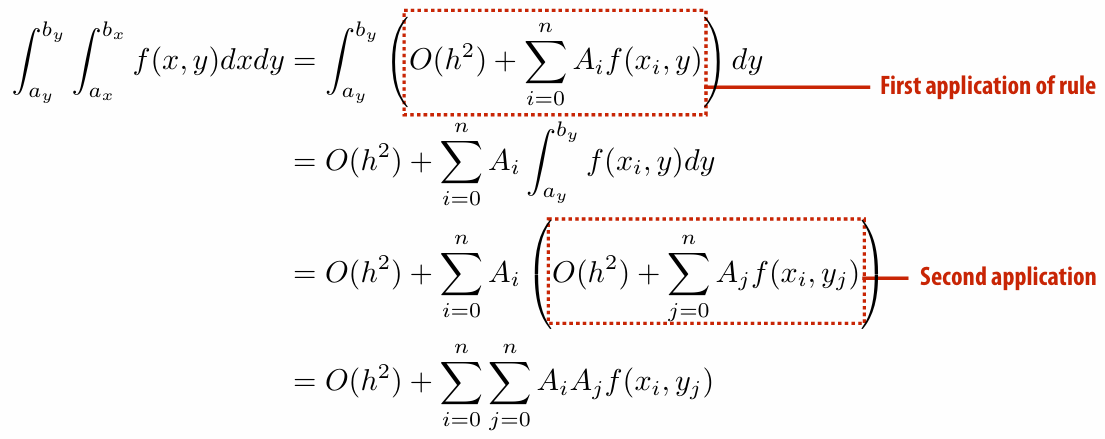
Error is still O(h^2), but work now is
How about k dimensions?
let
5.1.3 Curse of Dimensionality for Trapezoid Rule
How much does it cost to apply the trapezoid rule as we go up in dimension?
1D:
2D:
…
kD:
For many problems in graphics (like rendering), k is very, very big (e.g., tens or hundreds or thousands). Applying trapezoid rule does not scale!
5.1.4 Sampling from Discrete Probability Distributions
To randomly select an event, select
Here
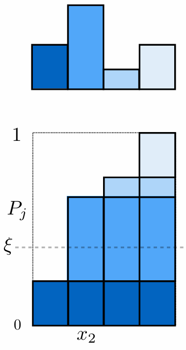
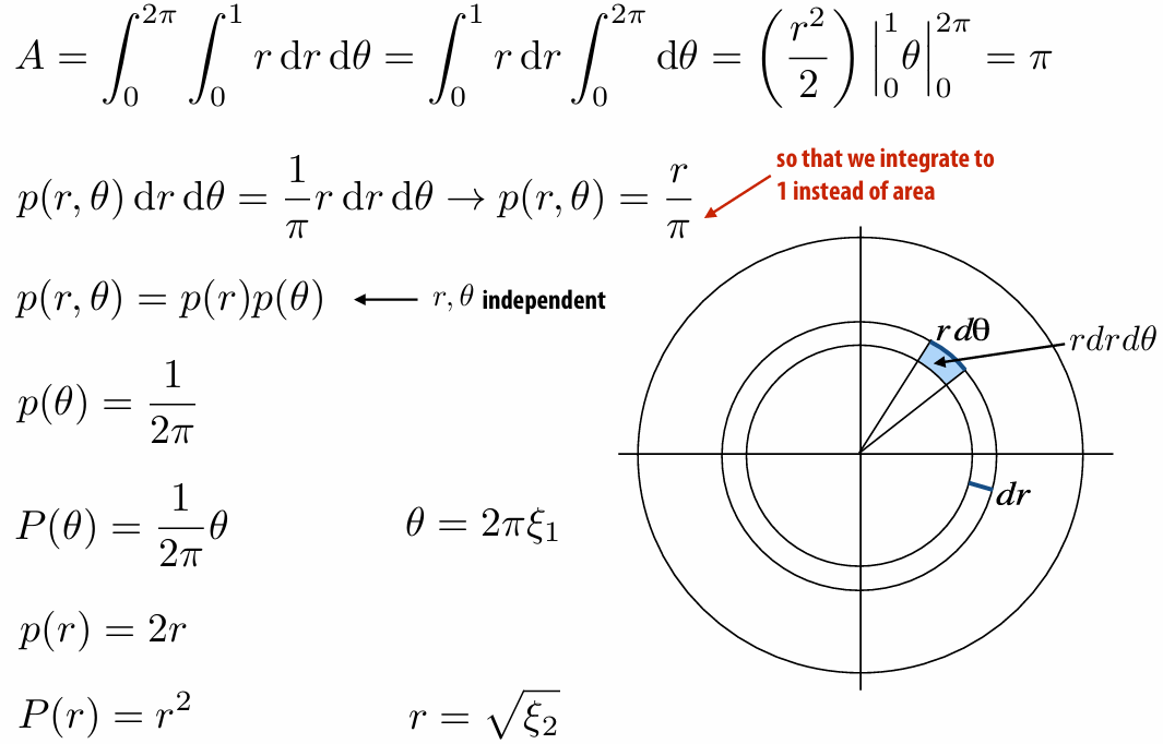
5.1.5 Sampling Continuous Random Variables using the Inversion Method
Cumulative probability distribution function
We must know integral of
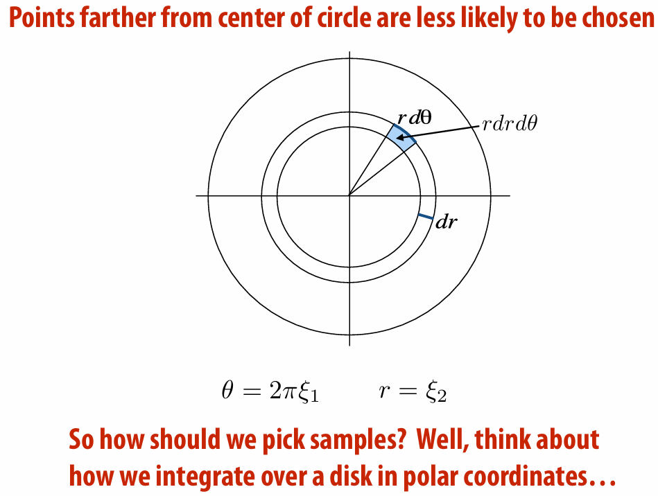
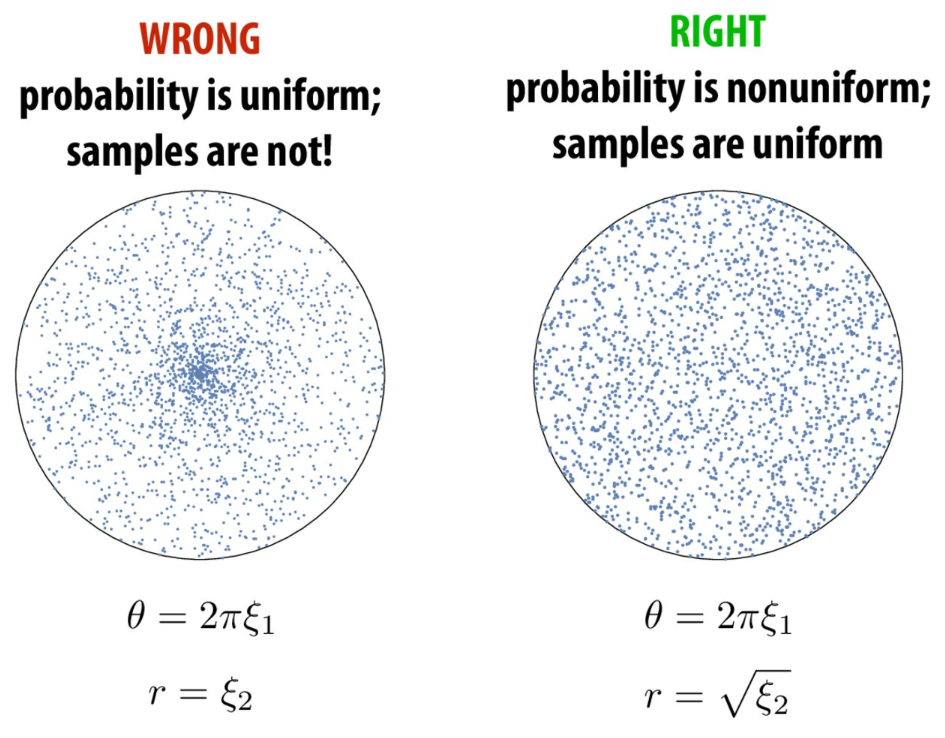
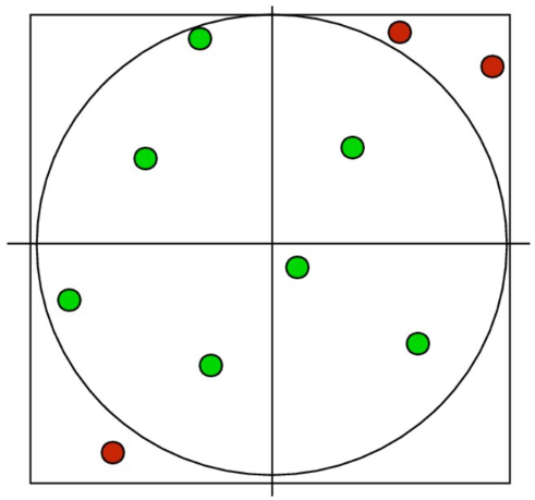
First try: uniformly sampling unit circle
*For the second line:
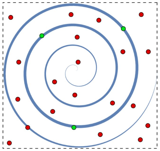
5.1.6 Rejection Sampling
5.2 Monte Carlo Rendering
5.2.1 Expected Value and Variance
Expected value:
Variance:
5.2.2 Law of Large Number
For any random variable, the average value of
The variance is always linear in
5.2.3 Biasing
To get the accurate integration, we should divide the
5.2.4 Importance Sampling

Sample the important area more. Remember divide the probability.
5.2.5 Monte Carlo Integration
According to law of large number, we know no matter how hard the integral is, we can always get the right image by taking more samples.
Keep in mind three key ideas:
Expected Value: what value do we get on average?
Variance: what’s the expected deviation from the average?
Importance Sampling: how do we (correctly) take more samples in more important regions?
The essence of integration is "function's accumulation on area", Monte Carlo Integration convert it into "average value of random sampling
The
The standard error is independent of dimensionality and only depends on the random samples used:
5.2.6 Russian Roulette
Randomly terminate the recursive integral of rendering equation.
5.3 Variance Reduction
Keep in mind: You can’t reduce variance of the integrand! Can only reduce variance of an estimator.
5.3.1 Estimator
An “estimator” is a formula used to approximate an integral, like the Monte Carlo estimator.

5.3.2 Bias & Consistency
Two important things to ask about an estimator
it consistent?
Is it biased?
Consistency: “converges to the correct answer”:
Unbiased: “estimate is correct on average”:
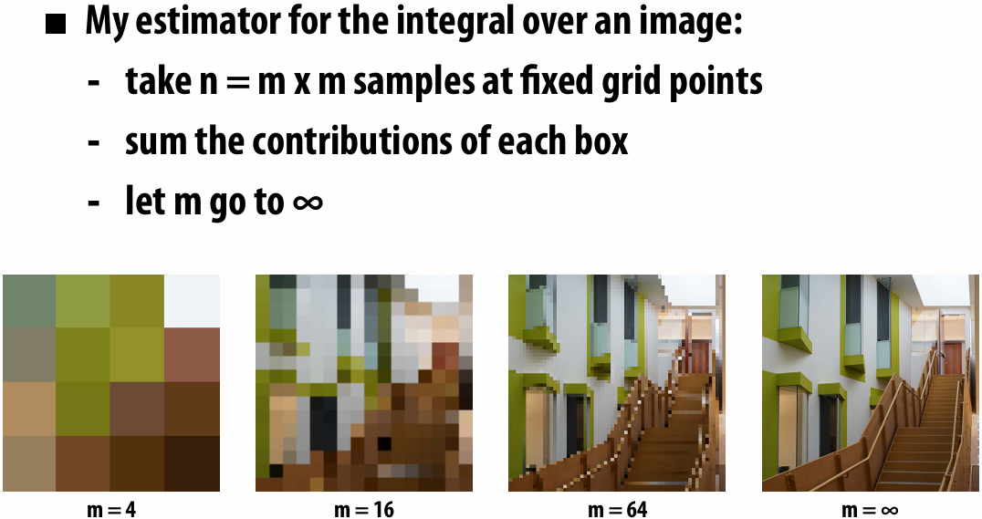
Example (Consistent but biased):
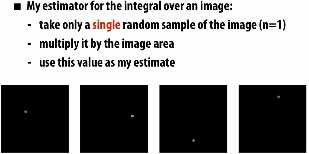
Example (Inconsistent but unbiased):
Rasterization and Path Tracing are neither consistent and unbiased.
Light has a very “spiky” distribution, how can we sample the lights more?
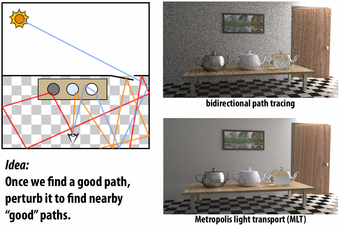
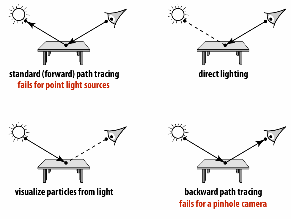
5.3.3 Bidirectional Path Tracing

Idea: connect paths from light, eye (“bidirectional”)
Example (path length is 2):
5.3.4 Metropolis-Hastings Algorithm (MH)
Good path can be hard to find!
Basic idea: prefer to take steps that increase sample value

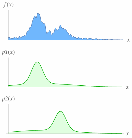
5.3.5 Multiple Importance Sampling
5.3.6 Sampling Patterns & Variance Reduction
How do we sample our function in the first place?
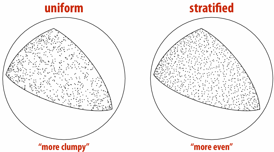
Stratified Sampling
Split into n bins, pick uniformly in each bin


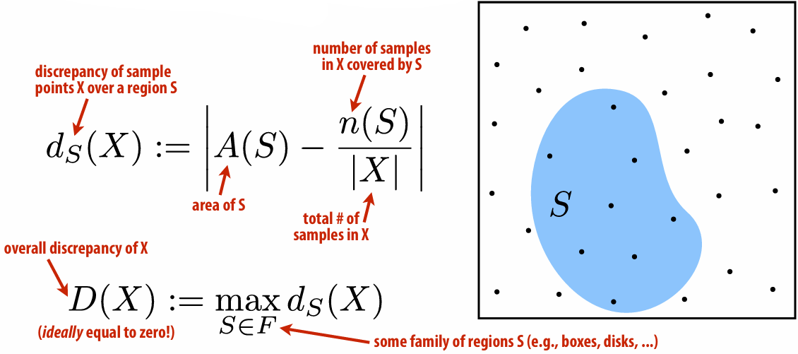
Low-Discrepancy Sampling: Number of samples should be proportional to area
*
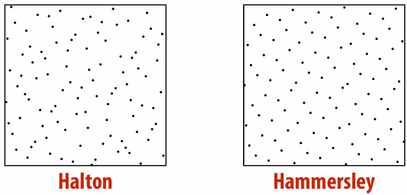
Hammersley & Halton Points:
First define radical inverse
Halton points in k-dimensions:
Hammersley sequence is
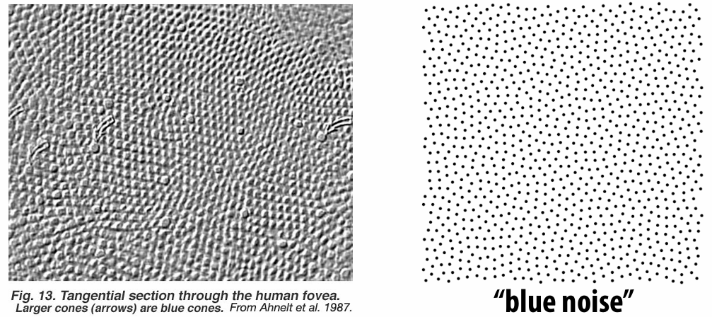
Blue Noise: Can observe that monkey retina exhibits blue noise pattern
…
6. Animation
6.1 Keyframe
6.1.1 Keyframing
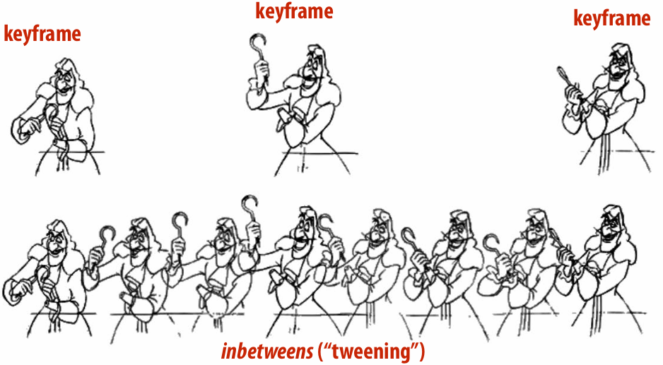
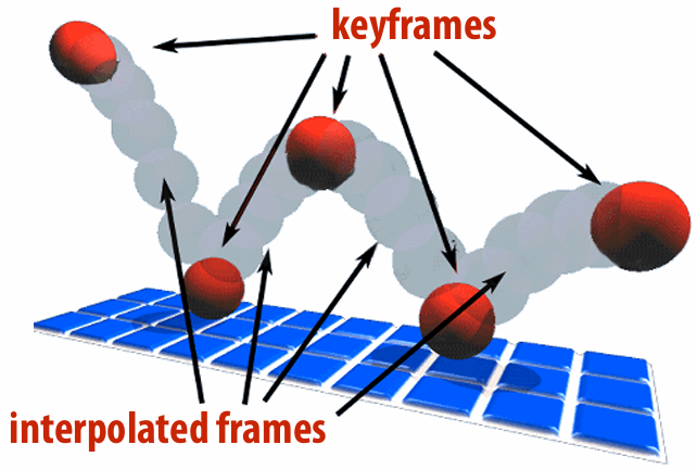
Specify important events only and computer fills in the rest via interpolation/approximation.
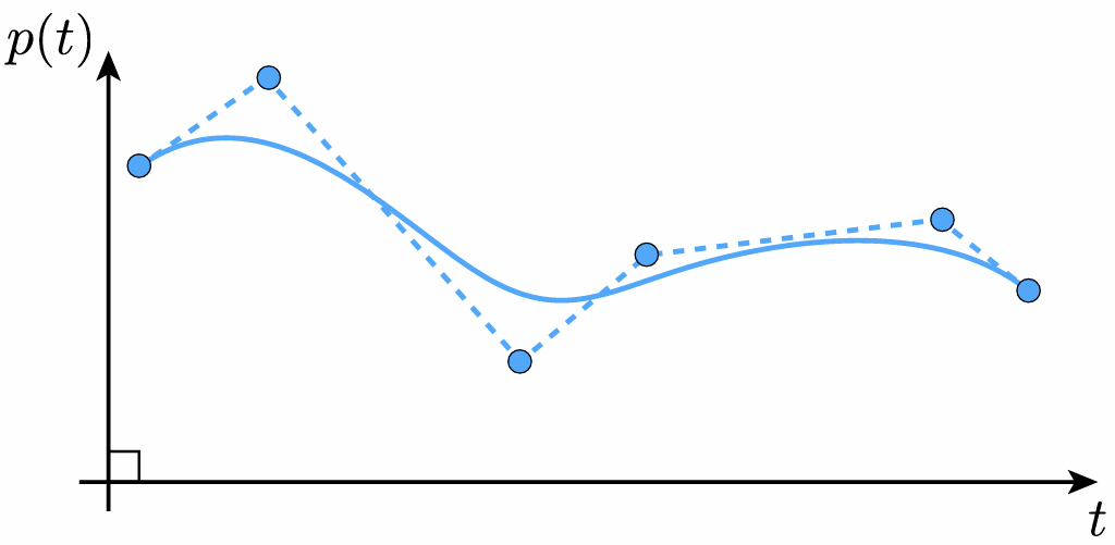
6.1.2 Spline Interpolation
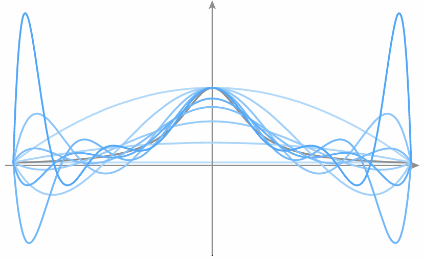
Runge Phenomenon: Tempting to use higher-degree polynomials, in order to get higher-order continuity, but can lead to oscillation, ultimately worse approximation.
6.1.3 Natural Splines
For each interval, want polynomial “piece” pi to interpolate data (e.g., keyframes) at both endpoints:
Want tangents to agree at endpoints (“C1 continuity”):
Also want curvature to agree at endpoints (“C2 continuity”):
Degree of freedom:
6.1.4 Hermite/Bézier Spline

6.1.5 Catmull-Rom Spline
Use the difference of neighbors to define tangent.
Details: Scotty3D_Benky/assignments/A4/T1-splines.md at main · tbbbk/Scotty3D_Benky
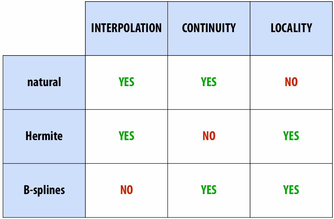
6.1.6 Evaluation of Spline
INTERPOLATION: spline passes exactly through data points
CONTINUITY: at least twice differentiable everywhere
LOCALITY: moving one control point doesn’t affect whole curve
6.2 Dynamics
6.2.1 Inverse Kinematics
Set a goal and use algorithm (like grad descent) to come up with a plausible motion.
*Detail: Scotty3D_Benky/assignments/A4/T2-skeleton.md at main · tbbbk/Scotty3D_Benky
6.2.2 Animation EquationF
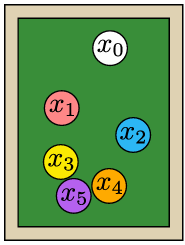
6.2.3 Generalized Config
Collect all points all into a single vector of generalized coordinates:

6.2.3 Ordinary Differential Equation (ODE)
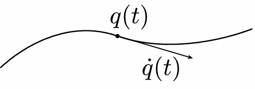
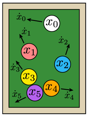
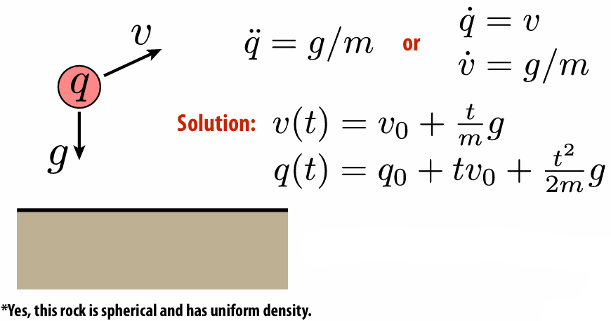
Many dynamical systems can be described via an ordinary differential equation (ODE) in generalized coordinates:
Example:
6.2.4 Lagrangian Mechanics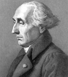
Write down kinetic energy
Write down potential energy
Write down Lagrangian
Dynamics then given by Euler-Lagrange equation:
6.2.5 Particle Systems
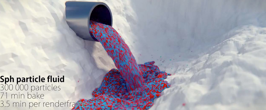
We model phenomenon as large collection of particles
How can we solve all these things numerically?
6.2.6 Forward/Backward Euler
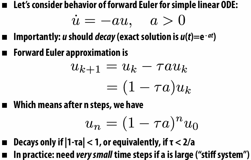
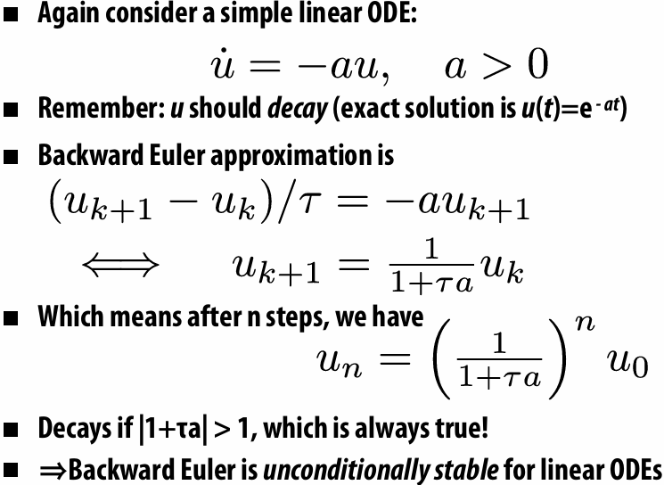
We can use the difference to replace derivatives.
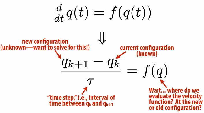
Forward Euler

But this is very unstable!
Backward Euler

But it is unconditionally stable!
6.2.7 Symplectic Euler
Backward Euler was stable, but we also saw (empirically) that it exibits numerical damping (damping not found in original eqn.). Nice alternative is symplectic Euler:
update velocity using current configuration
update configuration using new velocity
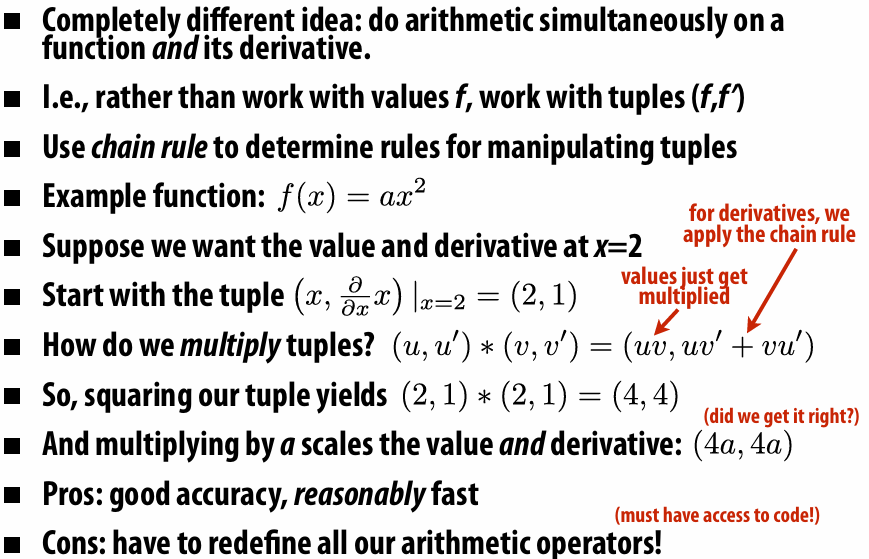
6.2.8 Automatic Differentiation
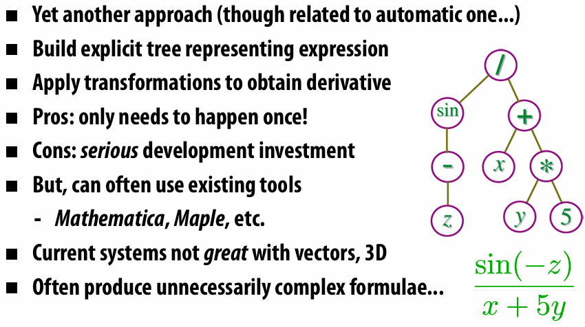
6.2.9 Symbolic Differentiation
6.2.10 Geometric Differentiation
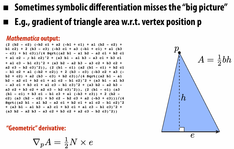
6.3 Partial Differential Equation (PDE)
ODE: Implicitly describe function in terms of its time derivatives
PDE: Also include spatial derivatives in implicit description
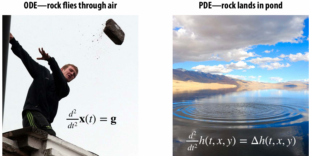
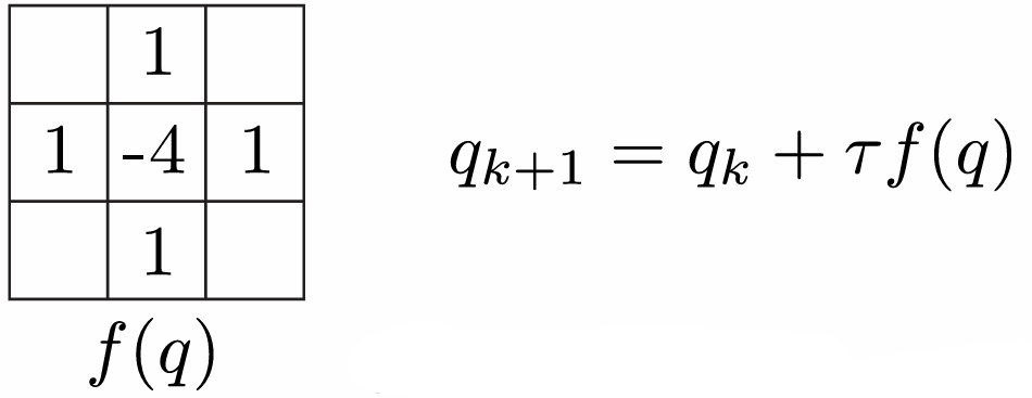
Solving a PDE looks like “take weighted combination of neighbors to get velocity (...and add a little velocity each time)”
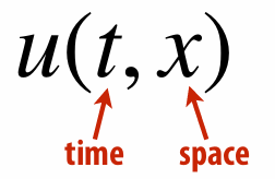
6.3.1 Definition of a PDE
Want to solve for a function of time and space
Example: nonlinear / higher order ⇒ HARDER TO SOLVE!

6.3.2 Lagrangian vs. Eulerian
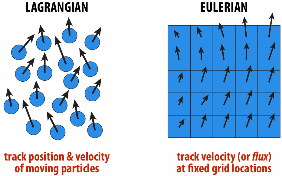
Trade-Offs:
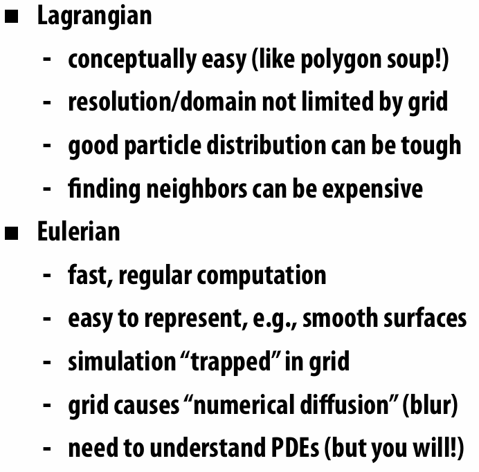
Of course, no reason you have to choose just one! You can mix them!
6.3.3 The Laplace Operator
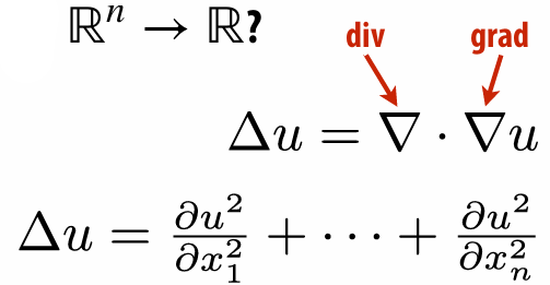
…
I sincerely do not understand the PDE well, orz.
